Heaps and priority queues

Many programs never need their data in full sorted order; they only need, again and again, the most urgent item: the next event in a simulation, the closest unvisited vertex in a shortest-path search, the job with the earliest deadline, the smallest head among a dozen sorted files. A priority queue is the abstract data type for exactly that, and the binary heap is the structure that implements it best in practice: a complete binary tree stored in a plain array, with insert and extract in O(log n), a look at the top in O(1) and the whole queue built from n items in Θ(n). This page defines the priority queue, compares its implementations, derives every heap operation together with the invariant it restores, proves the linear-time build, sorts with a heap, widens the tree into d-ary heaps, adds the decrease-key operation that Dijkstra's and Prim's algorithms need, and checks everything against Python's heapq. Afterwards you will be able to trace any heap operation by hand on the tree and on the array, implement and test a heap yourself, and choose between heapq, an indexed heap, lazy deletion and a sorted container for a real task. It builds on Trees and traversals and uses the comparison counts of Asymptotic analysis.

The structures need only the standard library; to run the plots and the notebook install the base group, add the structures group for the comparison with sortedcontainers and the graphs group for the check against NetworkX.

Intuition

Picture a large company drawn as an organisation chart in which every manager is senior to each of their direct reports. Nothing is promised about two colleagues side by side, or about people in different departments, yet one fact is certain: the most senior person sits at the top. When that person leaves, nobody re-ranks the whole company. The more senior of the two deputies moves up, then the more senior of that deputy's reports moves up into the gap, and so on down a single line of the chart. A newcomer joins at the bottom and is promoted past their manager, again and again, only while they outrank them. Each change touches one path from the top to the bottom, and the path of a balanced chart of n people is only about log2 n people long.

That chart is a heap. It keeps just enough order to answer "who is first?" instantly and to repair itself after a change along one path, which is far cheaper than keeping everybody sorted. A priority queue needs nothing more.

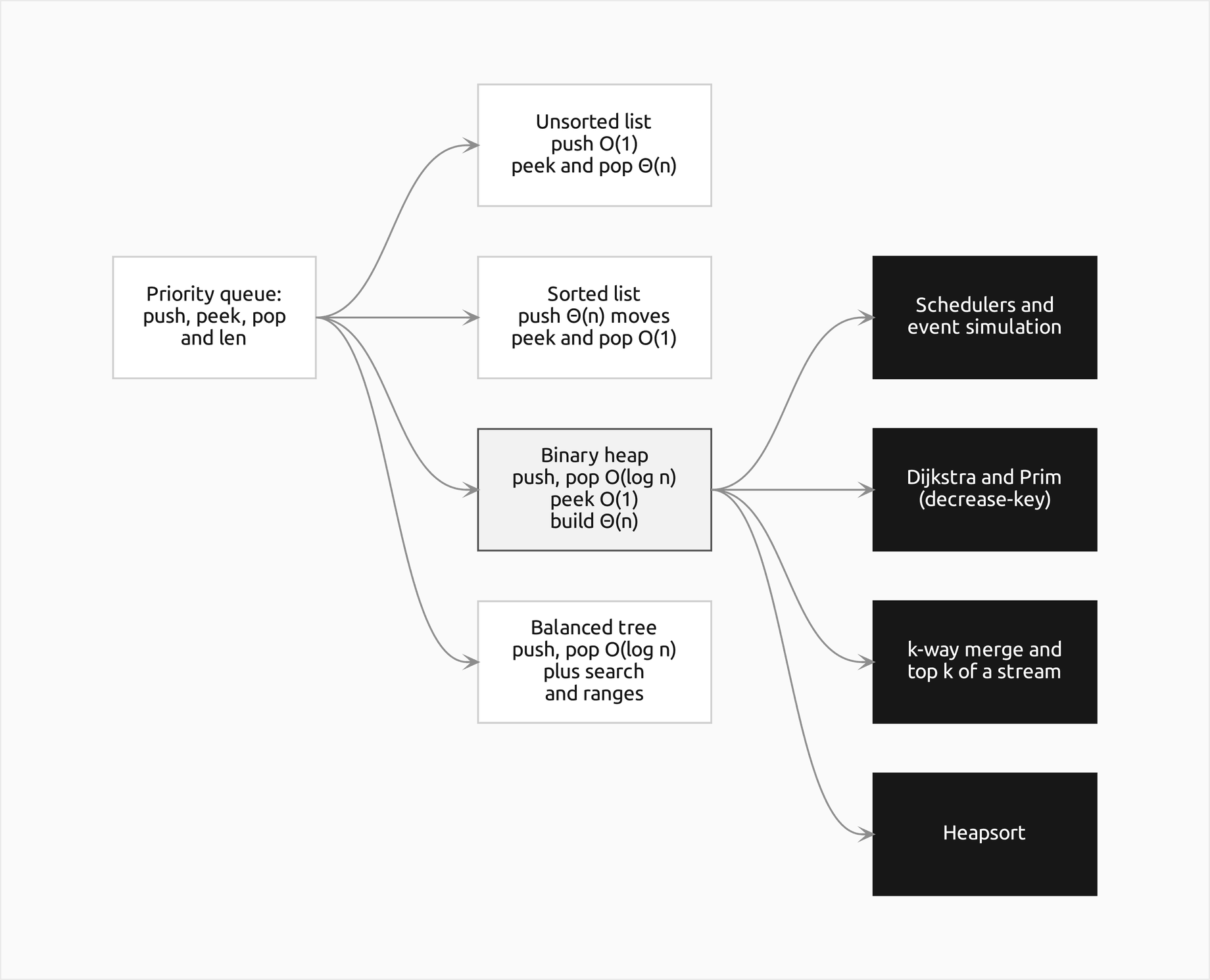
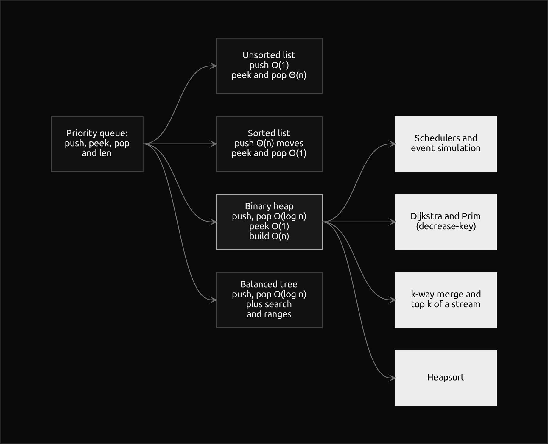
The diagram shows the abstract data type on the left, four ways to implement it in the middle and, in the filled boxes on the right, the jobs a heap does in this page and elsewhere in the handbook. The heap, outlined, is the only implementation that makes both push and pop logarithmic while keeping peek constant and the build linear.

How it works

The priority queue abstract data type

A priority queue holds items with priorities and offers four operations:

• push(x) adds an item.
• peek() returns an item of highest priority without removing it.
• pop() removes and returns an item of highest priority.
• len() says how many items remain.

Highest priority means smallest key in a min-priority queue and largest key in a max-priority queue; everything below is written for the min version, and the max version swaps every comparison. Two further operations matter for graph algorithms and schedulers: changing the priority of an item already queued (decrease-key when it can only improve), and removing an arbitrary item. Building the queue from n items at once is a useful extra. Nothing else is promised: a priority queue does not search, does not list its items in order, and does not say which of several equal keys comes out first. Those omissions are what make it cheaper than a sorted structure.

Four implementations

The same contract can be met in very different ways, and each choice moves the cost to a different operation:

• An unsorted list pushes by appending in O(1), but peek and pop must scan every item, Θ(n).
• A sorted list keeps the highest-priority item at one end, so peek and pop are O(1). Push finds its place by binary search in O(log n) comparisons, but then every item after that place shifts by one slot, Θ(n) moves in the worst case and n/2 on average.
• A binary heap does push and pop in O(log n) comparisons and swaps, peek in O(1) and builds from n items in Θ(n).
• A balanced search tree, such as an AVL or red-black tree, does push and pop in O(log n) as well, with a larger constant and more memory per item. In exchange it keeps all items in order, so it also answers searches, ranges and both ends at once.

The heap wins whenever only the top matters, which is why every standard library ships one. The section on cost measures all four on the same workload.

The binary heap

A binary heap is a binary tree with two properties. The shape property says the tree is complete: every level is full except possibly the last, which is filled from the left with no gaps. The order property, called the heap property, says every node's key is at most the keys of its children in a min-heap, or at least them in a max-heap:

The property is local, between a node and its parent, yet by following parents upward it implies that every node's key is at most every key in its subtree, so the minimum is at the root. It says nothing about siblings or cousins. That is the essential difference from a binary search tree, whose property orders a node against its whole left and right subtrees:

The two properties look alike but promise very different things, as the same keys arranged both ways show.

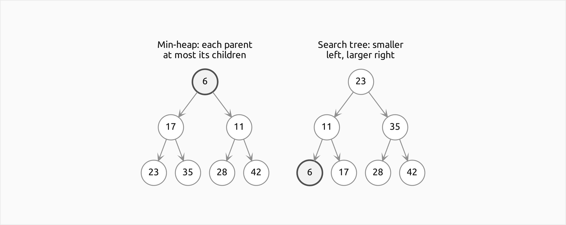
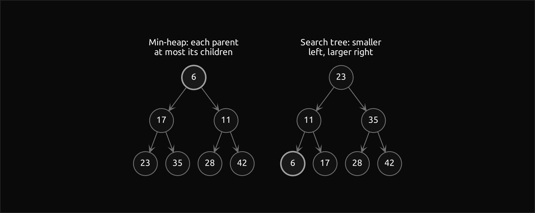
Both trees hold the same seven keys and have the same shape, with the minimum outlined. The heap answers "what is the smallest key?" at its root, but finding any other key means looking everywhere, because 17 sits left of 11 and nothing tells a search which way to go. The search tree finds any key along one path and lists the keys in order, but its minimum is at the end of the leftmost path and its shape depends on the order of insertions. A heap's shape never does: being complete, a heap of n keys always has height ⌊log2 n⌋, since a complete tree of height h holds at least one node on its last level and at most a full one:

A max-heap is the mirror image: every parent at least its children and the maximum at the root. The package expresses the choice as an Order object, MIN or MAX, that answers one question, whether item a must sit above item b. Only the strict test is ever asked, so equal keys never count as out of order and never swap.

Storing the tree in an array

A complete tree needs no pointers. Number the nodes level by level from left to right, starting at 0 at the root, and store node i in slot i of a Python list. The level structure turns into arithmetic: the children of node i sit at 2i + 1 and 2i + 2, and its parent at ⌊(i − 1)/2⌋.

For the heap built in the worked example, the arithmetic around index 1 looks like this:

Reading the array from left to right is a level-order walk of the tree, so the tree is never stored at all: it is a way of reading the array. Because the array has no gaps, the shape property holds automatically, and every operation below only has to repair the order property.

Two more facts follow from the numbering. Node i lies on level ⌊log2(i + 1)⌋, and it has a child exactly when 2i + 1 < n, so the leaves are the second half of the array:

Many books store the root at position 1 and leave slot 0 empty, which makes the formulas one step shorter:

In that layout the leaves are the positions ⌊n/2⌋ + 1 to n. The two layouts are the same arithmetic shifted by one position, p = i + 1:

The off-by-one comes from mixing them. Using the 1-based parent ⌊i/2⌋ on a 0-based Python list sends index 4 to index 2, its cousin, instead of index 1; using the 1-based children 2i and 2i + 1 makes the root its own left child. Likewise the 1-based loop "from ⌊n/2⌋ down to 1" over the internal nodes, copied onto a 0-based list, never visits the root at index 0. In 0-based terms the last node with a child is ⌊n/2⌋ − 1. Pick one layout and convert positions only at the boundary; the package uses 0-based indices throughout and keeps the 1-based formulas in layout.py only for comparison.

Insert: sift-up

To push x, append it at the end of the array. That is the only slot that keeps the tree complete. The new item may now be smaller than its parent, the one place where the order can be broken, so sift-up repairs it: while the item is smaller than its parent, swap the two and continue from the parent's slot.

The loop is correct because of an invariant: before every iteration, the array is a heap except that the item at the current index may be smaller than its parent. A swap moves the item up one level. Its new child, the old parent, was at most every key below it, so the subtree just left behind is in order, and the old parent is smaller than its other child too, so nothing breaks below. The only possible violation is again between the item and its new parent. The loop ends at the root or at a parent that is not larger, and either way the heap property holds everywhere. The path to the root has ⌊log2 n⌋ edges, so a push costs at most that many comparisons and swaps.

The pushed key, outlined while it moves and filled where it settles, climbs from A[10] past 30 and 15, which move down one level each and are outlined, and stops below 9. Only the three nodes on its path were examined.

Extract: sift-down

To pop, take the root, which is the answer. The tree must lose a node, and the only node it can lose while staying complete is the last one, so the last item moves into the root's slot and the array shrinks by one. That item came from the bottom and is usually large, so sift-down repairs the order: compare the two children of the item, take the smaller one, and if it is smaller than the item, swap them and continue from the child's slot.

The invariant now reads: both subtrees of the current index are heaps, and only the item there may be larger than its children. Promoting the smaller child is essential. That child becomes the parent of its former sibling, and it is at most that sibling, so the sibling's side stays in order; promoting the larger child would put it above a smaller sibling and break the heap. After the swap the only possible violation is between the item and its new children, one level lower. The loop ends at a leaf or where the item is at most both children. Each level costs two comparisons, one between the children and one against the smaller child, so a pop makes at most 2⌊log2 n⌋ comparisons and ⌊log2 n⌋ swaps.

The root 9 leaves, the last item 30 takes its place and sinks: 13 and 15, the smaller child at each level, move up. At A[4] its only child is 33, which is larger, so 30 stops there.

The version above is the textbook one, called classic here. Python's heapq uses a variant that saves comparisons: since the moved item almost always belongs near the bottom again, it first walks the hole all the way down to a leaf, promoting the smaller child at every level with one comparison per level, and only then sifts the item up from that leaf, which rarely takes more than a step or two. The package calls it leaf-first and implements both; sift_down_leaf_first also copies heapq's tie rule, so its arrays agree with heapq's exactly. In heapq's own source the names are the other way round: _siftdown moves an item towards the root and _siftup towards the leaves.

Peek, replace and pushpop

Peek returns A[0] without changing anything, O(1). Two combined operations each do a push and a pop for the price of one sift:

• replace(x) returns the root and puts x in its place, then sifts x down. It returns the old root even when x is smaller, so the result can be larger than the new item. This is a pop followed by a push.
• pushpop(x) is a push followed by a pop. If x is not larger than the root, x itself would come straight back out, so it is returned after a single comparison and the heap is untouched; otherwise the root is returned and x replaces it as in replace.

Both are the core of streaming algorithms: a merge replaces the head of the run it just consumed, and a top-k filter replaces its worst kept item whenever a better one arrives.

Removing any position and changing a priority

Removing the item at index i works like a pop at that position: the last item fills the hole and the array shrinks. The newcomer came from elsewhere in the tree, so it can be out of order in either direction, but only in one. If it is smaller than its new parent, it is also smaller than the children there, which were at least the removed item, which was at least that parent; then it must climb, and sift-up repairs it. Otherwise it may be larger than a child and must sink. The package's restore tries sift-up first and falls back to sift-down, one of which does nothing. Forgetting the sift-up case is a classic bug; the worked example has an instance.

Changing the priority of the item at index i is the same repair: write the new key and restore. A smaller key in a min-heap climbs, a larger one sinks. Both operations need the index of the item, which a plain heap does not know; finding it by scanning costs Θ(n). The indexed heap below removes that cost.

Building a heap from the bottom up

Given n items in an array, n pushes would build a heap in O(n log n). The bottom-up method, due to Floyd, does it in Θ(n). Every leaf is already a heap of one item, and the leaves are the second half of the array. So walk the internal nodes from the last one, ⌊n/2⌋ − 1, back to the root, and sift each one down.

The loop invariant is that before node i is processed, every node with a larger index is the root of a heap. Then both subtrees of i are heaps, which is exactly the precondition of sift-down, and afterwards i is the root of a heap too. When the loop has processed index 0, the whole array is a heap. The order matters: processing nodes from the root downwards would sift a node before its subtrees are heaps, and the result is not a heap.

In each frame the keys that moved up along the path of the sift-down are outlined and the key that sank is filled where it settled; in the first frame the filled keys are the two whose sift-down moved nothing. Most of the work is done near the bottom, where the subtrees are small; only the last sift-down starts from the root. Why that makes the total linear is the subject of the cost section.

Heapsort

A heap sorts in place. Build a max-heap over the whole array; its root is the largest item and belongs in the last slot. Swap it there, shrink the heap by one so that the slot is no longer part of it, and sift the new root down within the smaller heap. Repeat until the heap has one item.

The invariant after every pass is that the first end slots form a max-heap, the slots after them hold the largest items in sorted order, and no heap item is larger than a finished item. The swap moves the largest heap item to the front of the finished tail, which keeps the tail sorted; the sift-down restores the heap on the shrunk prefix and must not look past it, or it pulls finished items back in. Ascending order needs a max-heap for exactly this reason: the item removed in each pass belongs at the end. A min-heap used the same way produces descending order.

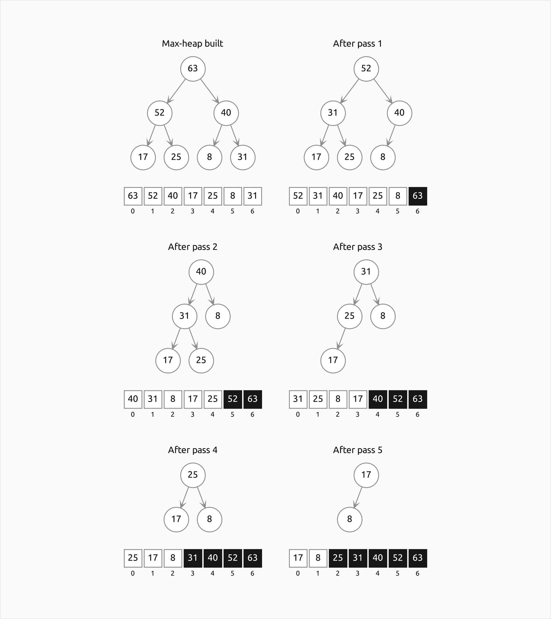
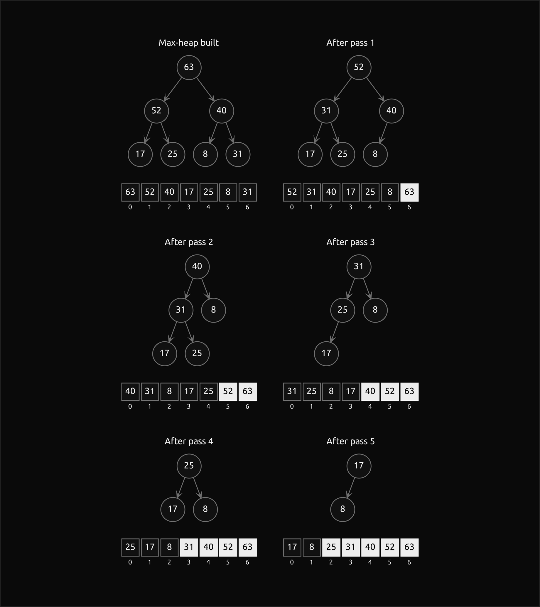
Each pass moves one more item into the filled tail and leaves a smaller heap in front of it. The last pass, not drawn, leaves 8 alone in the heap, already in place.

Heapsort runs in O(n log n) in the worst case and O(1) extra space, but it is not stable: equal keys can change their relative order, because the swap in each pass sends an item from the root across the whole heap. Sorting the five records 5a, 3a, 5b, 3b and 5c by their numbers alone, heapsort returns 3a, 3b, 5b, 5c, 5a, while a stable sort such as Python's sorted or merge sort keeps 5a, 5b, 5c in input order.

d-ary heaps

Nothing forces two children per node. In a d-ary heap, node i has the children d·i + 1 to d·i + d and the parent ⌊(i − 1)/d⌋:

A wider tree is shallower, with height about log n / log d:

Sift-up compares once per level, so it gets cheaper as d grows. Sift-down must find the smallest of up to d children, d − 1 comparisons, and compare it with the item, so it costs up to d per level and gets more expensive:

A workload dominated by pushes and decrease-keys, which both sift up, wants a larger d; one dominated by pops wants a small one. Four is a popular compromise: the four children of a node are adjacent in memory, often in one cache line.

Indexed heaps and decrease-key

Dijkstra's shortest paths and Prim's minimum spanning tree keep every unfinished vertex in a priority queue keyed by its tentative distance, and they lower a vertex's key whenever a shorter route to it appears. That decrease-key operation needs to find the vertex in the heap. An indexed heap keeps a map from each item to its current array position, alongside a map from each item to its priority. Every swap updates the two positions involved, so the map stays exact, and decrease-key becomes: look up the position in O(1), lower the priority, sift up, O(log n). The same map gives remove(item) and change_priority(item) in O(log n) for any item, and x in heap in O(1). The validity check for this structure, check_indexed_heap, compares the map with the array in both directions before checking the order.

Lazy deletion

Python's heapq has no decrease-key and no position map, and code built on it uses a different idea. When a priority changes, leave the old entry where it is, mark it as removed in O(1), and push a new entry with the new priority. When a marked entry later reaches the top, discard it and pop again. A dictionary from item to its current entry tells live entries from stale ones. Every stale entry is pushed once and popped once, so the extra work is paid for by the pushes that created it, but the heap can grow to the number of updates instead of the number of items. LazyPriorityQueue implements the pattern on heapq; its entries are (priority, sequence number, item) so that equal priorities leave in insertion order and the items themselves are never compared. Dijkstra written this way does not even need the marks: an entry whose priority is larger than the vertex's current distance is out of date.

Cost

Every operation

For a binary heap of n items:

• peek: O(1).
• push: at most ⌊log2 n⌋ comparisons and swaps, worst case. On random keys a new item climbs only a level or two on average, because half of all nodes are leaves and most keys belong near the bottom.
• pop, replace and pushpop: at most 2⌊log2 n⌋ comparisons and ⌊log2 n⌋ swaps with the classic sift-down, worst case; the item moved to the root usually sinks almost to the bottom, so the average is close to the worst case. The leaf-first variant needs about log2 n comparisons.
• remove at a known index and change a priority: O(log n), one of the two sifts.
• search for a key, or remove one whose index is unknown: Θ(n), because the heap property cannot steer a search.
• build from n items: Θ(n) bottom-up, proved next, against Θ(n log n) in the worst case for n pushes.
• merging two heaps of sizes m and n: Θ(m + n) by building a new heap from both arrays. Heaps designed for fast merging (binomial, pairing and Fibonacci heaps) trade the simple array for linked nodes.

All bounds are worst case unless stated otherwise; nothing here is amortized. That matters for real-time uses such as event loops and network schedulers: every single operation, not just their average, finishes within O(log n).

Why building bottom-up takes linear time

The sift-down started at node i can only move down, so it stops after at most height(i) levels, where height(i) is the length of the longest path from i to a leaf. In a complete tree that longest path is the leftmost one, and the node h levels down it is (i + 1)·2^h − 1, which exists as long as (i + 1)·2^h ≤ n. Counting nodes by height then becomes counting multiples:

Half the nodes are leaves and do no work, a quarter have height 1 and do at most one level, and so on: few nodes have long paths. The total work T(n) of the build is at most a constant c times the sum of the heights. The textbook route bounds that sum with the count of nodes of each height and a geometric series:

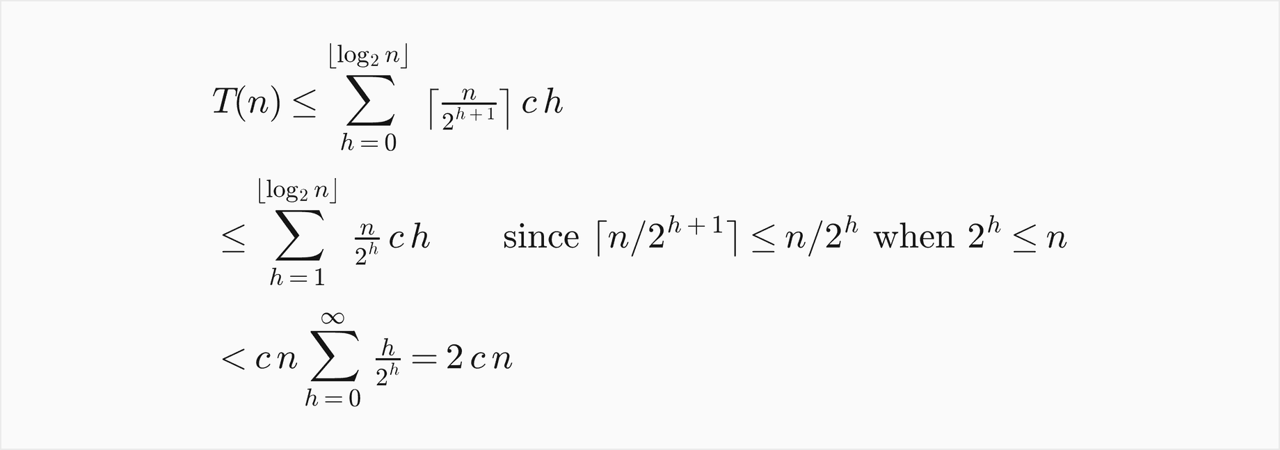
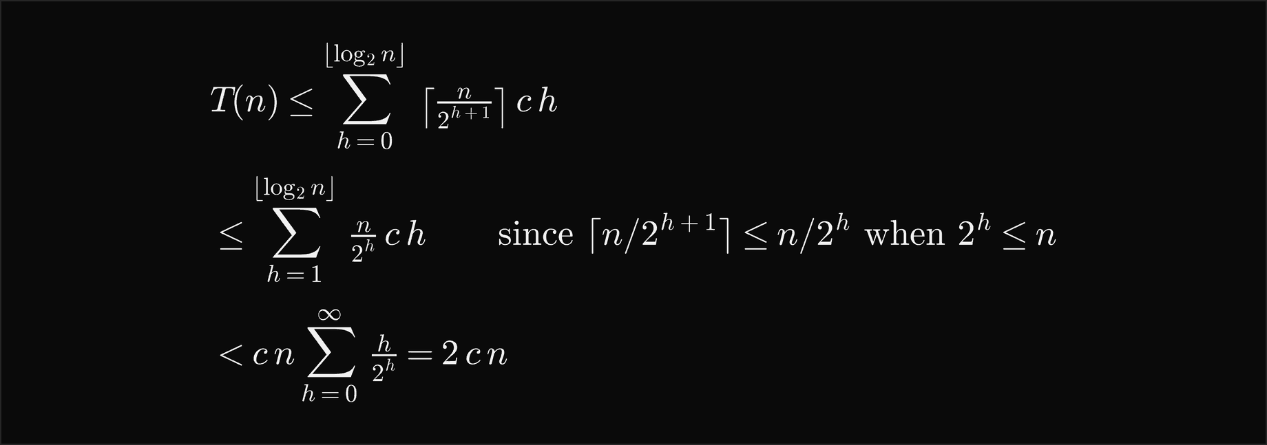
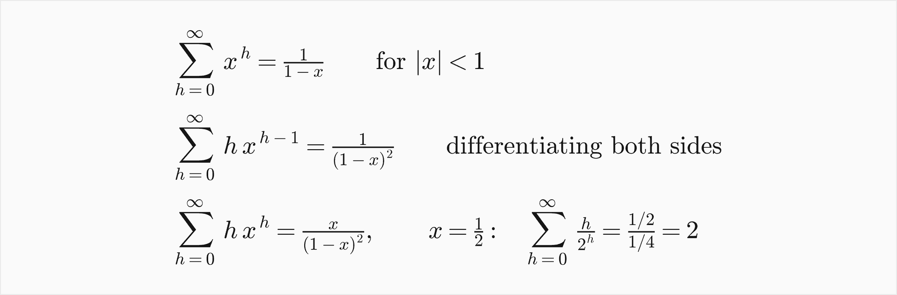
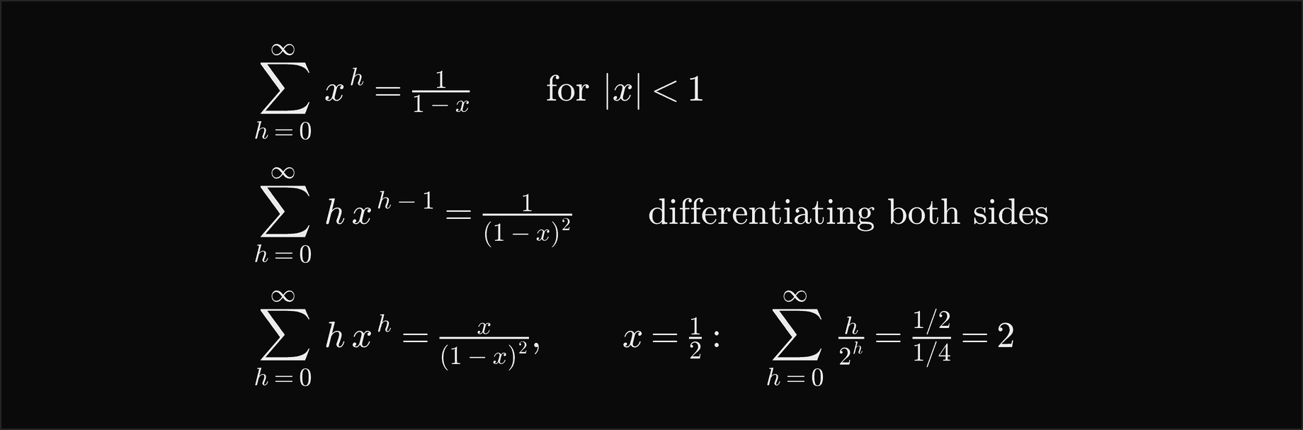
The infinite sum comes from differentiating the geometric series:

The sum of heights can also be computed exactly. Adding up height(i) is the same as adding up, for every k ≥ 1, the number of nodes whose height is at least k, and that number is ⌊n/2^k⌋. Writing n in binary with digits b_j, each digit 2^j contributes 2^(j−1) + 2^(j−2) + ... + 1 = 2^j − 1 to those floors:

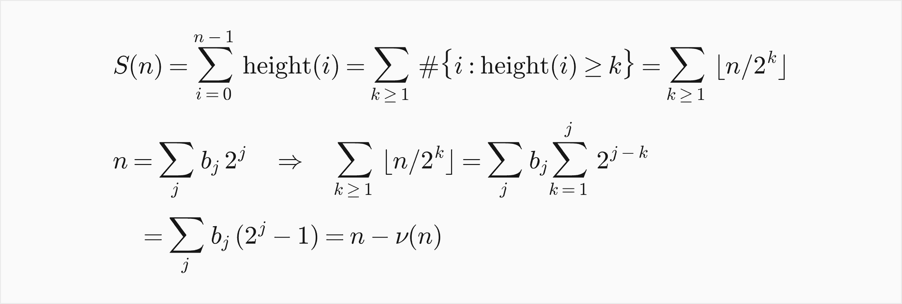
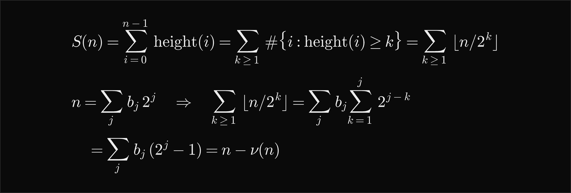
Here ν(n) is the number of ones in the binary form of n. The sum of heights is n − ν(n), always less than n; for the ten keys of the worked example it is 10 − 2 = 8. Each level of a classic sift-down swaps once and compares at most twice, which gives exact bounds for the whole build:

The build is linear in the worst case, with fewer than 2n comparisons for every input. Tests check both bounds on random, ascending and descending inputs.

Building by repeated insertion

Pushing the items one at a time costs, for the k-th push, at most the depth of slot k − 1, which is ⌊log2 k⌋. The worst case is reached exactly when every new key is smaller than everything before it, descending keys for a min-heap, because each one then climbs to the root with one successful comparison per level. Grouping the keys by level gives the exact total:

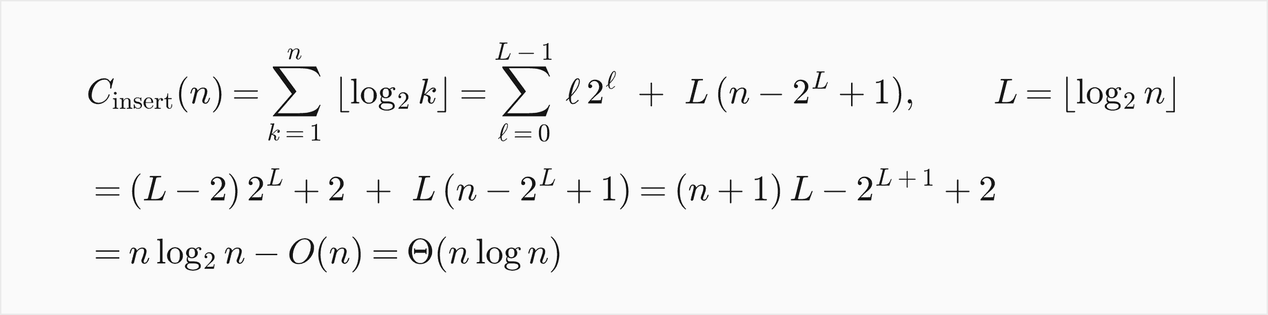
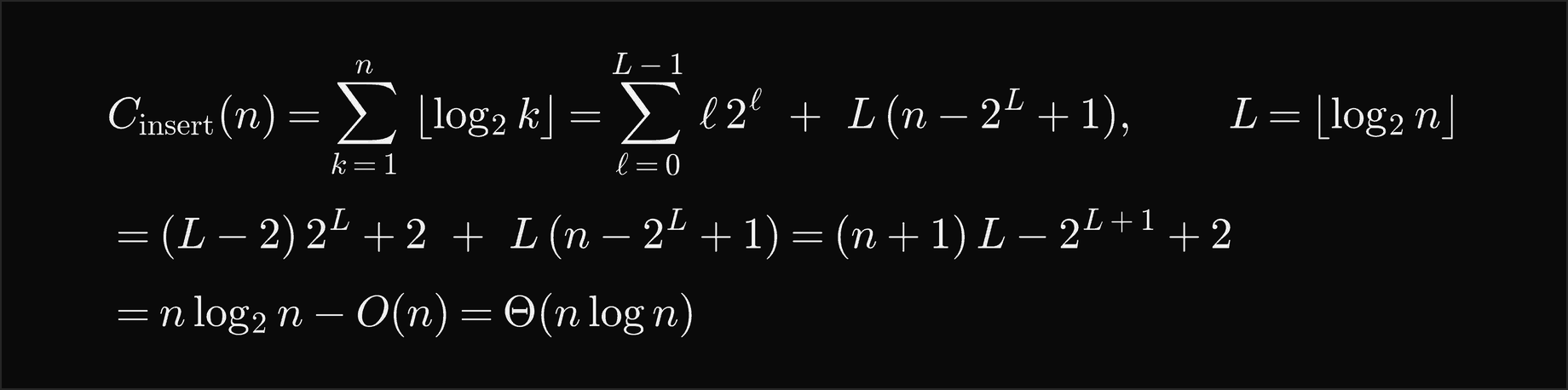
So repeated insertion is Θ(n log n) in the worst case, against Θ(n) for the bottom-up build. The difference comes from where the work happens: insertion makes the many nodes near the bottom travel the long way to the root, while the bottom-up build makes only the few nodes near the root travel far. On random input the picture changes: a random new key rarely climbs far, and exact average-case analyses show that both methods are linear on average, with repeated insertion slower by a constant factor.

Counted comparisons

The example build_and_sort_costs.py counts the comparisons of both methods for n from 16 to 16384, on descending keys (the worst case of insertion) and on random permutations (the mean of three seeds), and divides by n.

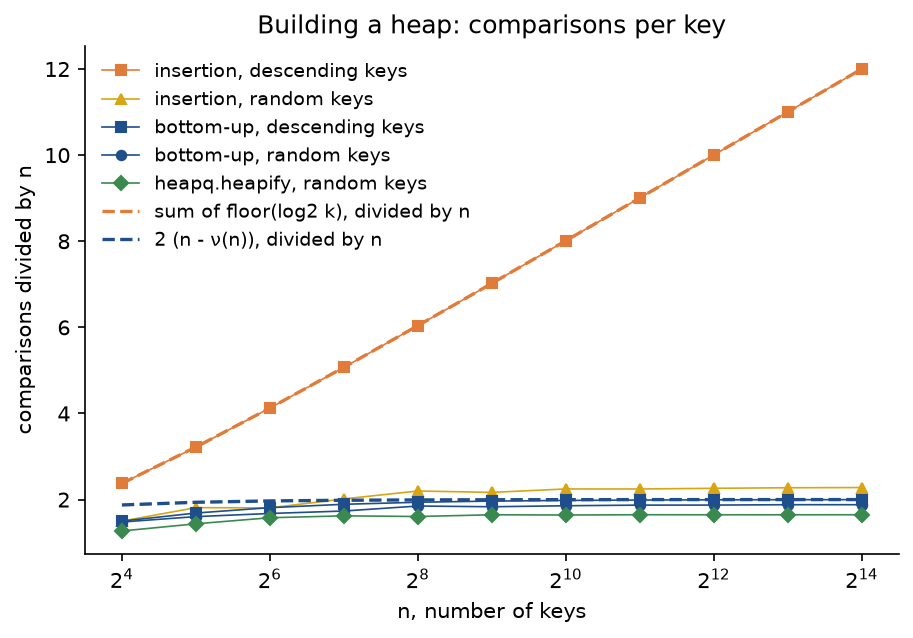
Per key, a linear cost is a flat line and an n log n cost a rising one. Insertion on descending keys climbs by one comparison per doubling of n and matches Σ⌊log2 k⌋ exactly at every size, 12.0010 per key at n = 16384. Every bottom-up curve stays under its bound: 1.9983 per key for descending keys, close to the worst case, and 1.8806 for random keys. Insertion on random keys also stays flat, at 2.2792 per key, which is the average-case linearity in numbers. heapq.heapify, the leaf-first build, needs only 1.6479.

Heapsort against merge sort

Heapsort makes at most 2(n − ν(n)) comparisons to build the max-heap and at most two per level for the sift-down after each of the n − 1 swaps, in a heap of k items for k from n − 1 down to 1:

Top-down merge sort never makes more than this many:

And no comparison sort can beat log2 n! comparisons in the worst case, since it must tell n! orders apart with yes or no answers:

Dividing every count by n log2 n shows the constants that the O-notation hides.

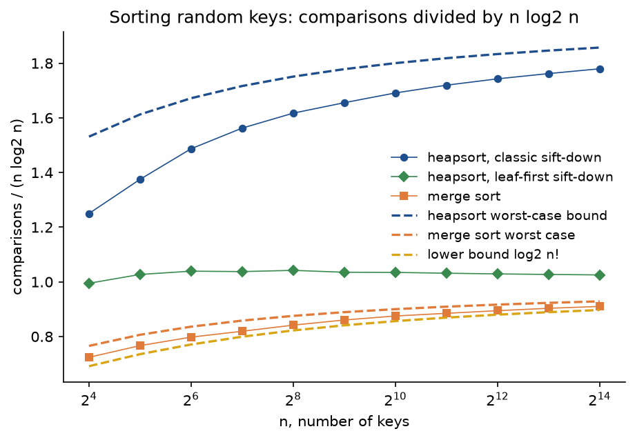
Classic heapsort makes nearly twice the comparisons of merge sort, 1.7795 n log2 n against 0.9100 at n = 16384, because each sift-down pays two comparisons per level and the item it sinks nearly always goes all the way. Switching to the leaf-first sift-down, known as bottom-up heapsort, brings it to 1.0253, close to merge sort and the lower bound of 0.8970. Heapsort's advantages are elsewhere: O(1) extra space and an O(n log n) worst case with no bad inputs. Its disadvantages are instability and poor memory locality, because a sift-down jumps from i to 2i + 1 across the array, which is why library sorts prefer merge sort variants such as Timsort or quicksort variants, and use heapsort as the fallback that bounds introsort's worst case.

The four implementations measured

The example queue_implementations.py pushes n random keys into each implementation and pops them all, counting comparisons and element moves (swaps for the heap and the unsorted list, one-slot shifts for the sorted list). The search tree is stood in for by SortedList from sortedcontainers, which keeps the items in a list of short sorted sublists rather than in a tree but offers the same logarithmic search; its comparisons are counted through wrapped keys, and its internal moves cannot be counted that way.

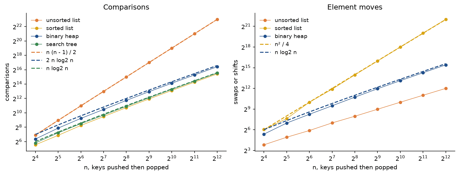
Comparisons alone flatter the sorted list: at n = 4096 it makes 43501 comparisons against the heap's 87186. The right panel shows its real cost: 4230454 elements shifted, n²/4 on average, against 43475 swaps for the heap, about 97 times fewer. The unsorted list makes exactly n(n − 1)/2 = 8386560 comparisons. Only the heap and the search tree are logarithmic in both measures.

Choosing d

The example dary_and_decrease_key.py measures one sift-up to the root and one pop in heaps of about 4096 keys for d from 2 to 16, and then runs Dijkstra's algorithm on two random graphs with n = 2000 vertices.

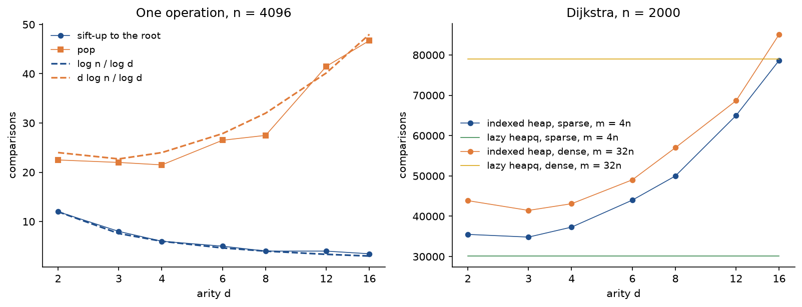
The left panel is the trade-off in the formulas: sift-up cost falls like log n / log d, pop cost grows like d log n / log d and is lowest around d = 3 or 4. For Dijkstra with n pops and up to m decrease-keys, the classical analysis balances the two by choosing d near m/n:

That analysis assumes every edge triggers a decrease-key. On random graphs with random weights only a small fraction do: 666 of 8000 edges on the sparse graph and 3783 of 64000 on the dense one. Pops dominate, and the best arity was 3 for both graphs, with 34832 and 41451 comparisons. The lazy version on heapq made fewer comparisons on the sparse graph, 30131, because its pops use the leaf-first sift-down, and many more on the dense one, 78962, because its heap held up to 4476 entries, 3796 of them stale when popped, against at most 1739 in the indexed heap.

Worked example

Every step below is printed by examples/worked_example.py and asserted by tests/test_worked_example.py. The keys are the ten integers 37, 22, 48, 15, 30, 41, 9, 26, 18 and 33, built into a min-heap.

Building the heap

The array has n = 10 slots, so the last node with a child is ⌊10/2⌋ − 1 = 4, and the build sifts down A[4], A[3], A[2], A[1] and A[0] in that order:

• A[4] = 30 has a single child, A[9] = 33. One comparison, 30 ≤ 33, and nothing moves.
• A[3] = 15 has the children 26 and 18. The first comparison picks the smaller child, 18 < 26; the second finds 15 ≤ 18. Nothing moves.
• A[2] = 48 has the children 41 and 9; 9 < 41, then 9 < 48, so 48 and 9 swap: [37, 22, 9, 15, 30, 41, 48, 26, 18, 33]. A[6] is a leaf, so the sift stops.
• A[1] = 22 has the children 15 and 30; 15 ≤ 30, then 15 < 22, swap: [37, 15, 9, 22, 30, 41, 48, 26, 18, 33]. At A[3] the children are 26 and 18; 18 < 26, then 18 < 22, swap: [37, 15, 9, 18, 30, 41, 48, 26, 22, 33].
• A[0] = 37 has the children 15 and 9; 9 < 15, then 9 < 37, swap: [9, 15, 37, 18, 30, 41, 48, 26, 22, 33]. At A[2] the children are 41 and 48; 41 ≤ 48, then 37 ≤ 41, and the sift stops.

The heap is [9, 15, 37, 18, 30, 41, 48, 26, 22, 33], after 13 comparisons and 4 swaps, within the bounds of 2(10 − 2) = 16 comparisons and 8 swaps. The first sift-down needed one comparison because its node had one child; every other level needed two.

Pushing 13

Push 13: it goes to A[10], whose parent is ⌊(10 − 1)/2⌋ = 4.

• 13 < 30 at A[4]: swap, giving [9, 15, 37, 18, 13, 41, 48, 26, 22, 33, 30].
• 13 < 15 at A[1]: swap, giving [9, 13, 37, 18, 15, 41, 48, 26, 22, 33, 30].
• 9 ≤ 13 at the root: stop.

Three comparisons and two swaps; 13 rose two levels and stopped one level below the root.

Popping the minimum

Pop returns 9. The last item, 30 at A[10], moves to the root and the array shrinks to ten slots: [30, 13, 37, 18, 15, 41, 48, 26, 22, 33].

• Children 13 and 37: 13 ≤ 37, and 13 < 30, so swap: [13, 30, 37, 18, 15, 41, 48, 26, 22, 33].
• At A[1], children 18 and 15: 15 < 18, and 15 < 30, so swap: [13, 15, 37, 18, 30, 41, 48, 26, 22, 33].
• At A[4], one child, 33: 30 ≤ 33, stop.

Five comparisons and two swaps. The heap now holds 13 where 9 was, and every other key is back where it was before the push.

Removing a position and changing a priority

Remove A[5] = 41. The last item, 33 at A[9], fills the hole: [13, 15, 37, 18, 30, 33, 48, 26, 22]. Its new parent is A[2] = 37, and 33 < 37, so it must climb, not sink: swap, giving [13, 15, 33, 18, 30, 37, 48, 26, 22], then 13 ≤ 33 at the root stops it. Two comparisons and one swap. A removal that only sifts down would have stopped at once, since 33 has no children at A[5], and left 33 below the larger 37.

Then raise the key at A[1] from 15 to 45. The restore tries sift-up first: 13 ≤ 45, so it does not climb. Sift-down then compares the children 18 and 30 and swaps with 18, giving [13, 18, 33, 45, 30, 37, 48, 26, 22]; at A[3] the children are 26 and 22, 22 < 26 and 22 < 45, swap: [13, 18, 33, 22, 30, 37, 48, 26, 45]. Five comparisons and two swaps.

Heapsort pass by pass

Heapsort sorts the seven keys 52, 17, 40, 63, 25, 8 and 31. The build sifts down A[2] (40 stays above 31), A[1] (17 swaps with 63) and A[0] (52 swaps with 63, then stays above 25), which takes 8 comparisons and 2 swaps and gives the max-heap [63, 52, 40, 17, 25, 8, 31]. Each pass then swaps the root with the last heap slot and sifts the new root down; the bar separates the heap from the finished tail:

• Pass 1: swap 63 and 31, sift 31 down past 52: [52, 31, 40, 17, 25, 8 | 63].
• Pass 2: swap 52 and 8, sift 8 down past 40: [40, 31, 8, 17, 25 | 52, 63].
• Pass 3: swap 40 and 25, sift 25 down past 31: [31, 25, 8, 17 | 40, 52, 63].
• Pass 4: swap 31 and 17, sift 17 down past 25: [25, 17, 8 | 31, 40, 52, 63].
• Pass 5: swap 25 and 8, sift 8 down past 17: [17, 8 | 25, 31, 40, 52, 63].
• Pass 6: swap 17 and 8; the heap has one item left: [8 | 17, 25, 31, 40, 52, 63].

The whole sort takes 20 comparisons and 13 swaps. In pass 3 the sift-down stops early, because after 25 swaps with 31 its only child at A[3] is 17; in pass 4 the swap with 25 lands 17 at A[1], whose child slot A[3] is already outside the heap.

The code

The package heaps_and_priority_queues is plain Python, one idea per module. Importing it needs only the standard library; Matplotlib is imported by plotting.py alone and sortedcontainers inside SearchTreeQueue.

• order.py holds the Order objects MIN and MAX, which answer whether one item must sit above another and carry the symbols traces print.
• layout.py holds the index arithmetic: parent, left and right for 0-based arrays, their 1-based counterparts, depth, height, node_height, first_leaf, the d-ary versions, and inorder and search_tree_array, which fill the same complete shape as a binary search tree for the comparison drawn above.
• counting.py holds OperationCounter, a dataclass with the fields comparisons, swaps and shifts that every algorithm accepts as an optional counter argument, and CountedKey, a wrapper that counts the less-than tests library code makes.
• trace.py holds the Step record (action, positions, keys, array snapshot, heap size, outcome, order), record, which appends a step to an optional trace list, and format_trace, which turns steps into the lines printed above.
• sifting.py holds sift_up, sift_down and sift_down_leaf_first, written with two helpers, outranks_at and swap_at, that count and trace every comparison and swap.
• building.py holds build_heap (bottom-up, either sift-down), build_by_insertion and the closed forms of the cost section.
• heap.py holds BinaryHeap with push, pop, peek, replace, pushpop, remove, update and drain.
• heapsort.py holds heapsort and heapsort_passes; mergesort.py holds the counted merge sort it is measured against.
• dary.py, indexed.py and lazy.py hold DaryHeap, IndexedHeap with decrease-key and LazyPriorityQueue on heapq; dijkstra.py runs shortest paths with each, as the workload that compares them.
• streams.py holds merge_sorted, a k-way merge, and stream_top_k; queues.py holds the priority queue protocol and its four implementations.
• invariants.py holds heap_violation, is_heap, check_heap, check_heapsort_state and check_indexed_heap, which tests run after every operation of long random operation sequences.
• workloads.py holds the worked example's keys, the seven keys compared as a heap and as a search tree, and seeded random inputs: permutations, keys with duplicates, operation sequences, graphs and sorted runs.
• drawing.py returns deterministic Graphviz text for heaps drawn as a tree above its array, single, before and after, or as a grid of stages; framing.py measures each frame (circle and cell sizes, caption lines, widths) and positions.py lays out each tree tidily, a parent centred over its children, so that every node is pinned where it belongs.
• comparisons.py puts heapq next to the package; pitfalls.py holds deliberately broken versions for the pitfalls below; plotting.py draws every plot in the handbook's colours.

Counting and tracing never change what the code does. A comparison inside sift-down is one call:

while (child := left(index)) < size:
    sibling = child + 1
    if sibling < size and outranks_at(
        array, sibling, child, order, counter, trace, "compare-children", size
    ):
        child = sibling
    if not outranks_at(array, child, index, order, counter, trace, "compare-child", size):
        break
    swap_at(array, index, child, counter, trace, size)
    index = child

The examples run in a few seconds each from the repository root:

• examples/worked_example.py prints every step of the worked example and writes the six generated diagram sources.
• examples/queue_implementations.py measures the four implementations of the abstract data type.
• examples/build_and_sort_costs.py measures both builds, heapsort and merge sort, and shows that heapsort is not stable.
• examples/dary_and_decrease_key.py measures d-ary heaps and Dijkstra with decrease-key and with lazy deletion.
• examples/common_mistakes.py runs every broken version from pitfalls.py next to the correct code.
• examples/compare_with_heapq.py checks the package against heapq and measures the top k of a stream.
• examples/practice.py prints fresh exercises with their solutions; --seed gives a new set.

python trees/heaps-and-priority-queues/examples/worked_example.py
python trees/heaps-and-priority-queues/examples/queue_implementations.py
python trees/heaps-and-priority-queues/examples/build_and_sort_costs.py
python trees/heaps-and-priority-queues/examples/dary_and_decrease_key.py
python trees/heaps-and-priority-queues/examples/common_mistakes.py
python trees/heaps-and-priority-queues/examples/compare_with_heapq.py
python trees/heaps-and-priority-queues/examples/practice.py --seed 7

The sample project, project/service_queue.py with its helper project/simulation.py, simulates a service desk with several servers event by event, entirely on priority queues. The event queue is a BinaryHeap ordered by time, holding the next arrival and one departure per busy server; the waiting room is a second BinaryHeap ordered by the scheduling policy. First come first served orders the room by arrival time, shortest job first by the service time, which is known on arrival. Jobs arrive as a Poisson process, and the default run simulates 200000 jobs at each of seven loads with three servers and exponential service times of mean 1, prints the mean, 95th percentile and maximum wait, the longest queue and the comparisons per heap operation, and saves two figures. Options --servers, --jobs, --loads, --service exponential|bimodal, --focus and --seed change the setup, and --figures writes the PNGs elsewhere; the default run takes about 15 seconds.

python trees/heaps-and-priority-queues/project/service_queue.py
python trees/heaps-and-priority-queues/project/service_queue.py --service bimodal --servers 2

For first come first served with exponential service, queueing theory gives the mean wait exactly. With arrival rate λ, service rate μ and c servers, the load is ρ:

and the Erlang C formula gives the probability of waiting and the mean wait in the queue:

The simulation agrees with it: at load 0.9 the mean wait under first come first served is 2.7510 against the predicted 2.7235, and at 0.8 it is 1.0786 against 1.0787.

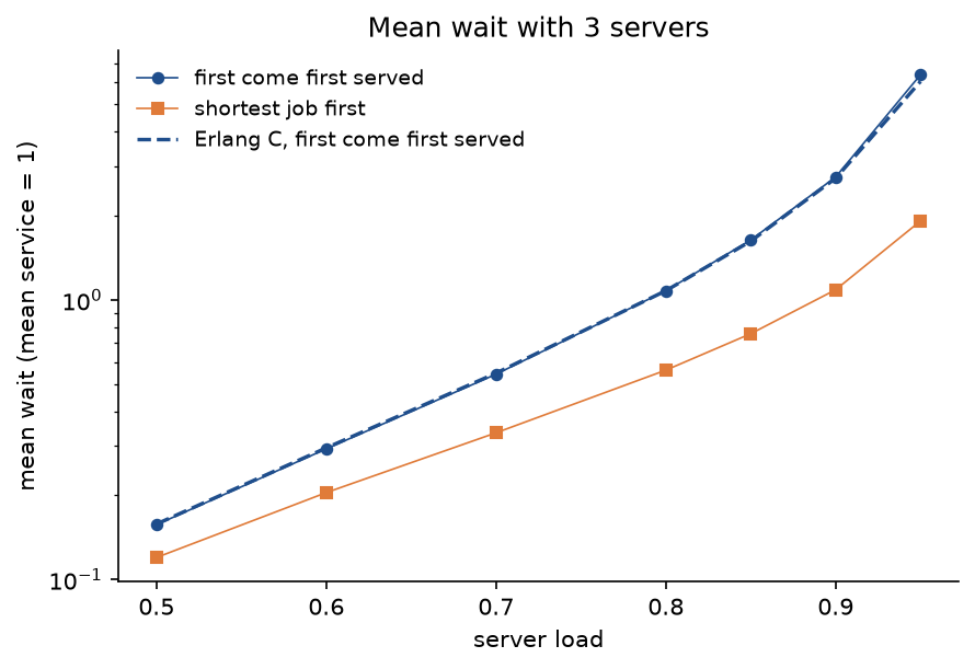
Serving short jobs first cuts the mean wait by a factor of about 2.5 at load 0.9, 1.0874 against 2.7510. The price is paid by long jobs:

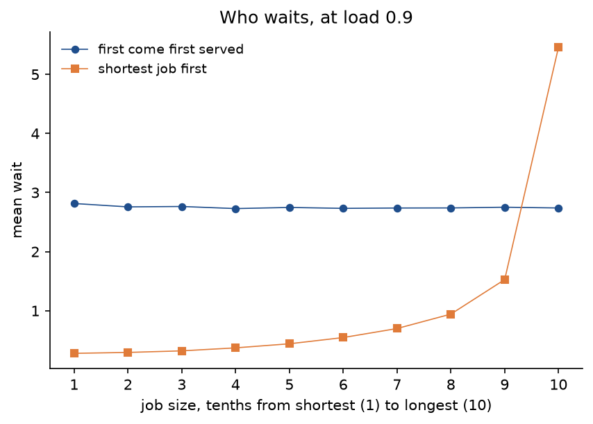
Under first come first served a job's wait does not depend on its size. Under shortest job first the shortest tenth waits 0.28 on average and the longest tenth 5.46, twice as long as under first come first served, and the longest wait of all grows from 27.86 to 236.35. Under heavier load a long job can starve while short ones keep overtaking it, which is why real schedulers add ageing, raising a waiting job's priority over time, a change of priority the indexed heap supports directly.

The notebook heaps_and_priority_queues.ipynb follows this page: the worked example step by step, the diagrams, the cost measurements, the comparison with heapq and the project's simulation at a few loads. The tests in tests check the worked example value by value, the invariants after thousands of random operations, the cost bounds on counts and the agreement with heapq, sortedcontainers and NetworkX, and run in a few seconds:

python -m pytest trees/heaps-and-priority-queues

All data are synthetic, generated from seeds by workloads.py and project/simulation.py, so nothing is downloaded and no licence is involved.

In practice

Python's heapq

Python's heapq module turns a plain list into a binary min-heap with heappush, heappop, heapify, heapreplace and heappushpop, written in C. The package's leaf-first BinaryHeap runs the same algorithm, and examples/compare_with_heapq.py shows that the two agree:

import heapq

from heaps_and_priority_queues import BinaryHeap, random_keys

keys = random_keys(1000, seed=1)
heap = BinaryHeap(variant="leaf-first")
mirror = []
for key in keys:
    heap.push(key)
    heapq.heappush(mirror, key)
    assert heap.array == mirror
assert heap.drain() == [heapq.heappop(mirror) for _ in range(len(keys))] == sorted(keys)

The pop order of both variants equals heapq's on every input, because both return the minimum each time. The arrays agree only for the leaf-first variant. heapq.heapify([27, 12, 12, 34, 19]) leaves [12, 12, 27, 34, 19], while the classic build leaves [12, 19, 12, 34, 27]: at the root the two children tie at 12, the classic sift-down takes the left one and heapq the right one. Both arrays are valid heaps; a heap is one of many valid arrangements, and tests should check the heap property and the pop order, not one particular array. Counted through wrapped keys, heapq makes exactly as many comparisons as the leaf-first variant: 6749 to build 4096 random keys against 7691 for the classic build, and 53036 for 4096 pushes and pops against 87145. In wall-clock time heapq is about 30 times faster than the pure-Python class, which is the usual gap between C and Python.

Max-heaps, ties and payloads

heapq is a min-heap. For numbers, negate on the way in and out. For anything without a meaningful negation, such as strings or tuples, wrap the items in a class whose less-than is reversed, as Descending in comparisons.py does; negating a string raises TypeError. Python 3.14 adds heapify_max, heappush_max, heappop_max, heapreplace_max and heappushpop_max to heapq.

Queued tasks usually carry a payload. Pushing (priority, task) tuples works until two priorities tie and Python compares the tasks, which raises TypeError for dictionaries and silently orders other objects by something meaningless. The standard fix is a counter between them, (priority, next(count), task): the count is unique, so the comparison never reaches the task, and equal priorities leave first in first out. TaskQueue and LazyPriorityQueue both do this.

Merging, nsmallest, nlargest and the top k of a stream

heapq.merge(*iterables) merges sorted inputs lazily with a heap of one entry per input, which is how sorted files too large for memory are combined. Each output item costs one replace in a heap of k entries:

The package's merge_sorted returns exactly what heapq.merge returns, and merging 8 sorted runs of 4346 items in total took 17288 comparisons against that bound of 26092.

heapq.nlargest(k, items) and heapq.nsmallest(k, items) return the k extreme items in order. For the k largest of a stream, keep a min-heap of the best k seen so far: its root is the worst of them, so each new item costs one comparison with the root, and only an item that beats the root costs a replace. Memory stays at k items however long the stream. When the stream arrives in random order, item i is among the best k so far with probability k/i, so the expected number of replacements grows only logarithmically:

Each replacement costs one sift-down in a heap of k items and every other item a single comparison with the root, which bounds the total:

Since R grows only like k ln(N/k), the first term dominates for long streams. The example compare_with_heapq.py measures R for two values of k:

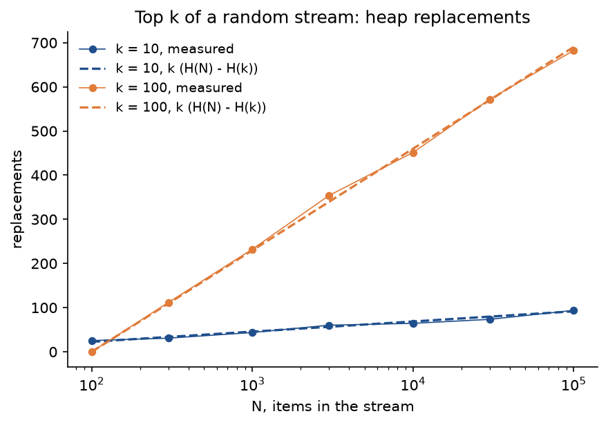
For k = 100 and N = 100000 the heap changed 682.4 times on average against the predicted 690.3: almost every item is rejected by a single comparison with the root. stream_top_k returns the same items as nlargest and nsmallest. CPython's nlargest uses the same idea for small k and calls sorted when k is at least the input size. When to use which:

• Use heapq for a priority queue of comparable items in Python, with the counter trick for payloads and lazy deletion for priority changes.
• Use an indexed heap when priorities change often and memory matters, as in a dense graph, or when you need remove(item) and membership tests.
• Use sortedcontainers.SortedList or a balanced search tree when you also need searches, ranges, both ends or ordered iteration.
• Use queue.PriorityQueue only for passing work between threads: it is heapq behind a lock.
• Use nlargest, nsmallest or a size-k heap for the top k of a stream, and sorted when k is close to n.

Elsewhere

Java's PriorityQueue, C++'s std::priority_queue (with std::make_heap, push_heap and pop_heap over any random-access container), Go's container/heap and Rust's BinaryHeap are all binary heaps in an array; C++ and Rust default to max-heaps, Java and Python to min-heaps. None offers decrease-key, and code that needs it uses lazy deletion or an indexed heap. Operating systems keep timers and runnable tasks in heap-like queues, network routers schedule packets with them, and event-driven simulators and game engines are built around one event queue like the project's. Libraries that need cache-efficient queues often use 4-ary heaps, and the Linux kernel's timer and scheduler code use other structures (timer wheels and red-black trees) when operations other than the minimum are frequent. Fibonacci heaps make decrease-key amortized O(1), which improves Dijkstra's bound to O(m + n log n) in theory, and pairing heaps come close in practice, but their pointers and constant factors usually lose to a binary or 4-ary heap.

Pitfalls

• Mixing 0-based and 1-based index formulas. On a 0-based list the parent of i is (i − 1) // 2, not i // 2, and the children are 2i + 1 and 2i + 2, not 2i and 2i + 1. With i // 2 a push into [10, 30, 20, 40] compares 25 with its cousin 20 instead of its parent 30 and leaves 25 below 30. Translate pseudocode written for 1-based arrays by shifting every position, as the conversion formula shows; examples/common_mistakes.py runs this and every following mistake.
• Building with the wrong loop. The internal nodes of a 0-based array are 0 to n // 2 − 1, visited from the last to the first. The 1-based loop from n // 2 down to 1 copied literally sifts one leaf for nothing and never sifts the root; walking from the root downwards sifts nodes before their subtrees are heaps; sifting down only the root restores a heap whose subtrees are already heaps but does not build one. On [44, 12, 31, 27, 18, 9] all three leave an invalid array.
• Comparing with the wrong child. Sift-down must compare the two children with each other first and swap with the smaller one. Looking only at the left child misses a smaller right child, and swapping with the first child smaller than the item, rather than the smallest, puts a larger child above its smaller sibling. When tracing by hand, write down both children at every level before deciding.
• Considering children beyond the heap. A child index must be below the current heap size, not below the length of the array. In heapsort the finished tail is still in the array, and a sift-down that ignores the shrunk size pulls finished items back into the heap: [52, 17, 40, 63, 25, 8, 31] comes out as [52, 63, 25, 31, 40, 17, 8].
• Using a min-heap for ascending heapsort. The item removed in each pass is swapped to the end of the heap, so a min-heap sorts in descending order. Ascending order needs a max-heap.
• Removing a position with sift-down only. The item that fills the hole can be smaller than its new parent; removing A[5] in the worked example needs a sift-up. Restore in both directions.
• Treating a heap as a search structure. Searching a heap or checking membership is Θ(n), and a sorted array is a heap but a heap is not a sorted array: only the root has a known rank. If you need search or order, use a search tree.
• Breaking a heapq list from outside. list.pop(0) returns the minimum but shifts every other item one slot left, which changes every parent-child pair; use heappop. Changing an item in place, or pushing onto a list that was never heapified, gives wrong pop orders without any error: after changing one priority inside [3, 8, 5, 12, 9, 7, 6] the pops come out as [3, 5, 6, 1, 7, 8, 12]. Call heapify after bulk changes, or use lazy deletion.
• Pushing tuples without a tie breaker. (priority, task) raises TypeError as soon as two priorities tie and the tasks cannot be compared. Put a counter in the middle.
• Negating keys that are not numbers. Negation makes a max-heap from heapq only for numbers; wrap other keys in a reversed comparison, or use the max-heap functions of Python 3.14.
• Expecting a particular array. Different correct implementations leave different valid arrays, as heapq.heapify and the classic build do. Test the heap property and the pop order instead.
• Expecting stability. Neither heapsort nor a heap pops equal keys in insertion order; add a counter to the key when the order of ties matters.

Further reading

• J. W. J. Williams, "Algorithm 232: Heapsort", Communications of the ACM 7(6), 347-348, 1964. The binary heap and heapsort.
• R. W. Floyd, "Algorithm 245: Treesort 3", Communications of the ACM 7(12), 701, 1964. The bottom-up construction in linear time.
• D. E. Knuth, The Art of Computer Programming, volume 3, Sorting and Searching, second edition, section 5.2.3, Addison-Wesley, 1998. Heapsort, its analysis and the leaf-first improvement.
• T. H. Cormen, C. E. Leiserson, R. L. Rivest and C. Stein, Introduction to Algorithms, fourth edition, chapter 6, MIT Press, 2022. Heaps, heapsort and priority queues with the linear-time build.
• R. Sedgewick and K. Wayne, Algorithms, fourth edition, section 2.4, Addison-Wesley, 2011. Priority queues, indexed priority queues and their applications.
• D. B. Johnson, "Priority queues with update and finding minimum spanning trees", Information Processing Letters 4(3), 53-57, 1975. d-ary heaps and the choice of d for graph algorithms.
• I. Wegener, "Bottom-up heapsort, a new variant of heapsort beating, on an average, quicksort (if n is not very small)", Theoretical Computer Science 118(1), 81-98, 1993.
• R. Hayward and C. McDiarmid, "Average case analysis of heap building by repeated insertion", Journal of Algorithms 12(1), 126-153, 1991.
• M. L. Fredman and R. E. Tarjan, "Fibonacci heaps and their uses in improved network optimization algorithms", Journal of the ACM 34(3), 596-615, 1987.
• D. H. Larkin, S. Sen and R. E. Tarjan, "A back-to-basics empirical study of priority queues", Proceedings of ALENEX, 61-72, 2014. Measures binary, d-ary, pairing and Fibonacci heaps and finds the simple ones hard to beat.
• The Python documentation of the heapq module, which includes the priority queue recipe with counters and lazy deletion.