Dynamic programming

Many problems that look as if they need a search through exponentially many candidates, every way to cut a rod, every subset of items that fits in a bag, every way to bracket a product of matrices, collapse into a few hundred small questions once you notice that the same smaller questions come up again and again. Dynamic programming answers each small question once, writes the answer down, and builds the answer to the big question from the stored ones. This page explains when that works (optimal substructure and overlapping subproblems), turns it into a four-step recipe, and applies the recipe to Fibonacci numbers in four ways, rod cutting, the 0/1 knapsack and matrix-chain multiplication, each traced cell by cell with its solution reconstructed. It compares memoization with tables, shows why the knapsack table is only pseudo-polynomial, shows where greedy choice fails and where it is optimal, and recasts every dynamic program as a shortest or longest path in a directed acyclic graph. Afterwards you will be able to design a dynamic program for a new problem, fill its table by hand in a valid order, recover the optimal solution and not just its value, and choose between functools.cache, a table and a library solver. It builds on Recursion and Recurrences and the master theorem; its sequel is Dynamic programming on sequences.

The algorithms need only the standard library; to run the plots and the notebook install the base group, and the graphs group for the checks against SciPy and NetworkX.

Intuition

Suppose you are packing for a hike with a bag that holds 8 kilograms and four items to choose from. You could try all sixteen subsets, but with forty items there would be more than a trillion. Instead, take a sheet of squared paper and answer smaller questions: what is the best you can carry using only the first item, if the bag held 0, 1, 2, ... 8 kilograms? Then using the first two items? To answer "the first two items with 6 kilograms of room" you need only two numbers already on the sheet: the best with the first item alone and 6 kilograms (leave the second item at home), and the best with the first item alone and 6 minus the second item's weight (pack it). Every cell is one comparison of two cells above it, and the last cell is the answer.

That is dynamic programming in one paragraph. Two properties make it possible. The best packing is made of best packings of smaller bags, so small answers can be trusted as building blocks (optimal substructure). And the same small questions are asked by many larger ones, so writing them down saves work (overlapping subproblems). Plain recursion has the first property but ignores the second, which is why it repeats itself:

The tree on the left computes F(5) by the definition F(n) = F(n − 1) + F(n − 2) and makes 15 calls; the amber ones recompute something a previous call already knew. The graph on the right has one vertex per distinct subproblem, six in all. Dynamic programming walks the graph, not the tree, and the gap between the two grows exponentially with n.

How it works

Optimal substructure and overlapping subproblems

An optimization problem has optimal substructure when an optimal solution consists of a first choice followed by optimal solutions of the subproblems that choice leaves behind. Then the value of a subproblem s satisfies a recurrence of this shape:

The argument that justifies it is always the same cut-and-paste: if the part of an optimal solution that solves a remaining subproblem were not itself optimal, swapping in a better solution of that subproblem would improve the whole, a contradiction. Richard Bellman, who named the method in the 1950s, called this the principle of optimality; "programming" meant planning, as in a production schedule.

Optimal substructure alone does not make a problem a dynamic program. Merge sort's halves are independent, so divide and conquer solves each once without storing anything. When one safe choice can be made before any subproblem is solved, a greedy algorithm needs only one subproblem. Dynamic programming is the right tool when the subproblems overlap: many different choices lead to the same smaller subproblem.

The three strategies share the same starting point and differ in how the subproblems relate. Divide and conquer and greedy algorithms have their own pages; this page is about the middle branch.

The subproblem graph

Draw one vertex per distinct subproblem and an edge from each subproblem to every subproblem its recurrence reads. Because every recurrence reads strictly smaller subproblems, the graph is acyclic. Plain recursion explores this graph as if it were a tree, so a vertex reachable along many paths is solved once per path. explore in subproblems.py builds the graph from a dependency rule, and recursion_tree_size counts what plain recursion would do on it: 465 calls for F(12) against 13 vertices.

A dynamic program solves every vertex once, and the work at a vertex is proportional to the number of subproblems it reads, so its running time is a sum over the graph:

Every cost on this page comes from this sum: count the subproblems, count the choices per subproblem, multiply.

Fibonacci four ways

The Fibonacci numbers are the smallest example with overlapping subproblems. With the convention used throughout this page,

Some books start the sequence at F(1) = 0 and F(2) = 1 instead, which shifts every index by one; check the convention before comparing answers.

Plain recursion (fib_naive) runs the definition. Its number of calls obeys the same recurrence plus one, and adding one to both sides turns it into the Fibonacci recurrence itself:

F(n) grows like a power of the golden ratio, so the calls do too:

F(25) takes 242785 calls this way.

Memoization (fib_memo) keeps the recurrence and adds a dictionary: before computing F(k), look it up; after computing it, store it. The package writes the mechanism out as a small class, Memo, whose call method is the whole idea:

def __call__(self, *key):
    self.counter.calls += 1
    if key in self.table:
        self.counter.hits += 1
        return self.table[key]
    self.depth += 1
    self.max_depth = max(self.max_depth, self.depth)
    try:
        value = self.rule(self, *key)
    finally:
        self.depth -= 1
    self.table[key] = value
    self.counter.cells += 1
    return value

The rule recurses through the memo, so every recursive call passes the check. Each value is computed once, and only the first call for each value recurses:

fib_cached does the same with functools.cache, whose cache_info() reports hits and misses; the counts match fib_memo call for call.

A table (fib_table) drops the recursion: fill F(0), F(1), ..., F(n) from left to right, so both values a cell reads are already there. Same n + 1 values, n − 1 additions, no call stack at all.

Two variables (fib_constant) notice that each cell is read only by the next two, so the table can shrink to the last two values: constant space. (Beyond dynamic programming, fib_doubling computes F(n) from F(k) and F(k + 1) at half the index in about log2 n steps; it is in the package for comparison.)

The recipe

Every dynamic program on this page, and most elsewhere, is designed in the same four steps.

1. Define the subproblems in words, precisely enough that a reader could compute one cell by hand: "r[j] is the best revenue from a rod of length j", "V[i][c] is the best value using the first i items with capacity c". Most failed attempts fail here, with a subproblem that forgets something the future depends on.
2. Write the recurrence: the best choice for a cell in terms of smaller cells, and the base cases that need no choice. Its correctness is the cut-and-paste argument above.
3. Choose an evaluation order in which every cell comes after the cells it reads, that is, a topological order of the subproblem graph. A memo finds one automatically by recursion; a table needs one written down, and a wrong one silently reads cells that are still empty.
4. Reconstruct the solution. The table holds values, not decisions, so store the winning choice of each cell next to it (or recompute it) and walk back from the answer.

Rod cutting

A rod of integer length n can be cut into pieces of integer lengths, and a piece of length i sells for a price p_i. Which cuts earn the most? A rod of length n has 2^(n − 1) ways to be cut, one for each subset of the n − 1 places a cut can go.

Subproblem: r(j), the best revenue from a rod of length j. Choice: the length i of the first piece. After cutting it, what remains is a rod of length j − i, which must itself be cut optimally (otherwise a better cut of the remainder would improve the whole). Uncut is the choice i = j:

Run as plain recursion (cut_rod_naive), each length calls every shorter length, and the count doubles with each unit of length:

The table (cut_rod_table) fills r[0], r[1], ..., r[n] in increasing order of length and stores in first[j] the first piece of a best cut. On a tie the shortest first piece wins, and ties are common: cutting 3 then 4 earns the same as 4 then 3. The reconstruction (reconstruct_cuts) reads first[n], cuts that piece off, and repeats on the remainder.

The tempting greedy rule, always cut the piece with the best price per unit of length, is implemented as greedy_by_density and fails on the worked example below: the best density can leave a remainder that sells badly.

The 0/1 knapsack

There are n items, item i with integer weight w_i and value v_i, and a bag of integer capacity W. Choose a subset of total weight at most W and the largest total value; each item is taken whole or left out, hence 0/1.

Subproblem: V[i][c], the best value using only the first i items with room c. Choice: whether item i goes in. If it stays out, the best is V[i − 1][c]; if it goes in, which needs w_i ≤ c, the rest of the bag must hold the best subset of the first i − 1 items within c − w_i:

The test is w_i ≤ c, not w_i < c: an item that exactly fills the remaining room does fit. The proof that V[n][W] is the optimum is induction on i: an optimal subset of the first i items either excludes item i, and is then optimal among the first i − 1 items, or includes it, and then the rest is an optimal subset of the first i − 1 items for the reduced room.

A cell reads only the row above it, so knapsack_table fills the table row by row; within a row any order works. Row 0 and column 0 are zero.

The backtrace (backtrace) walks from V[n][W] up to row 0. At row i, if the cell differs from the one above, item i must have been taken, so it is recorded and the room drops by w_i; otherwise it was left out. When both choices give the cell's value, leaving and taking are equally good, and the reported subset depends on a tie rule. The package's default rule, tie="leave", leaves the item out whenever the cell equals the one above; tie="take" puts it in whenever taking reaches the cell's value. Both report optimal subsets, possibly different ones, and the worked example has a tie at its final cell, so state the rule when you compare answers.

Greedy against the knapsack

If items can be cut, the knapsack becomes easy. Sort by value per unit of weight and take whole items until the next one does not fit, then the fraction of it that fills the bag:

An exchange argument proves it optimal: a solution holding less of a higher-ratio item and more of a lower-ratio one can trade equal weights between them without losing value, until it matches the greedy one. fractional_knapsack computes it with exact fractions.

For whole items the same rule can be arbitrarily bad. A light item with the best ratio can occupy just enough room to keep out an item worth nearly the whole capacity:

No other simple order is safe either; find_counterexample finds instances where ordering by value or by lightness loses too. Greedy fails for the 0/1 problem because taking an item is not a safe first choice: whether it was right depends on what else fits, which is exactly the subproblem the table remembers. The fractional optimum is still useful as an upper bound on the 0/1 optimum, the bound that branch and bound prunes with.

Matrix-chain multiplication

Multiplying a p by q matrix by a q by r matrix in the ordinary way takes one multiplication for each of q terms of each of p r entries:

A chain A1 A2 ... An, with Ai of shape p_(i−1) by p_i, can be multiplied in any order, since matrix multiplication is associative, and the orders can differ in cost by large factors. The number of orders is a Catalan number, which grows like 4^n:

Subproblem: m[i][j], the fewest multiplications for the product Ai ... Aj. Choice: the split k of the last product, (Ai ... Ak)(Ak+1 ... Aj), which costs the two halves plus one product of a p_(i−1) by p_k matrix with a p_k by p_j matrix. The halves must be multiplied optimally, or a better order for one half would improve the whole:

The subproblems overlap heavily: m[2][4] is read by m[1][4], m[2][5] and every longer chain containing it.

The evaluation order is the step that needs thought. Cell (i, j) reads cells (i, k) to its left in the same row and (k + 1, j) below it in the same column, all of them shorter chains. matrix_chain_order therefore fills the table by chain length, the diagonal just above the main diagonal first and the corner (1, n) last. Filling rows from the bottom up, each from left to right, is another valid order (order="rows"), and gives identical tables. Filling rows from the top down is not: it reads cells below that are still zero.

The split table s holds the best k for every chain. parenthesize reads the tree of the best order from it, splitting (1, n) at s[1][n] and each half at its own split, and format_order prints the tree with brackets. On a tie the smallest k wins.

Memoization against tabulation

Memoization and tabulation solve the same subproblems with the same recurrence; they differ in who chooses the order.

• Order. A memo lets the recursion discover a valid order: a subproblem is computed exactly when it is first needed. A table needs the order written down, and the order is part of the design: increasing length for rods, row by row for the knapsack, diagonal by diagonal for matrix chains.
• Which cells. A memo solves only the subproblems reachable from the question asked. In the knapsack with large weights that is a small fraction of the table, as the cost section measures. A table fills every cell, reachable or not, but pays no call overhead and touches memory in order.
• Recursion depth. A memoized recursion holds one level per pending subproblem: n levels for F(n), up to n for a rod of length n, n + 1 for n knapsack items. CPython stops at 1000 frames by default. The hand-written Memo uses two Python frames per level, so it fails near F(500); functools.cache wraps the function in C and reaches about twice as deep. Raising the limit with sys.setrecursionlimit only moves the wall and can crash the interpreter, so the package's library code never does it; a table has no depth at all.
• Space. A table can often forget rows it will never read again. The knapsack needs only the previous row, and it can even overwrite that row in place if the capacities are visited from high to low:

Visited from low to high, the cell for c would read a cell for c − w_i that already includes item i, which counts the item twice and solves the unbounded knapsack instead (unbounded_knapsack). The one-row version (knapsack_one_row) needs Θ(W) space instead of Θ(nW), but the table a backtrace needs is gone; recovering the subset then needs the choices stored separately, or a cleverer scheme such as Hirschberg's, covered for sequences in Dynamic programming on sequences. Fibonacci shrinks to two variables the same way. The matrix-chain table cannot shrink, because a cell reads its whole row and column.

Use a memo when the recurrence is easy to write and only part of the subproblem space matters, and when the depth is safe. Use a table when every cell is needed anyway, when the input is large enough for depth to matter, or when you want to save space by rolling rows.

Dynamic programming as paths in a DAG

Label every edge of the subproblem graph with the gain of the choice it stands for. Then a sequence of choices from the full problem to a base case is a path, its total gain is the path's weight, and the optimal value is the weight of the best path. A maximizing recurrence is a longest-path problem, a minimizing one a shortest-path problem, and since the graph is acyclic both are solved by relaxing the edges of each vertex in topological order:

Negative weights are harmless in a DAG, so a longest path is a shortest path with every weight negated, which is how dag_longest_paths in dag.py works. For rod cutting, a vertex is a remaining length and an edge from j to j − i cuts off a piece of length i:

Every path from 7 to 0 is a way to cut the rod, and the longest one, 14 + 17 = 31, is the best cut. The rod-cutting table computes the same thing from the other end: r[j] is the longest path from j to 0, filled for j from 0 upwards. The knapsack fits the same mould with a vertex (i, c) per cell and two edges per vertex (knapsack_dag), and so does line breaking in the sample project, as a shortest path. The same view explains Bellman-Ford, which is a dynamic program over paths of at most k edges; see Single-source shortest paths and Topological sorting. Counting problems are path counts in the same graphs: F(n + 1) is the number of ways to climb n stairs in steps of 1 and 2, which is the number of paths from n to 0 in the Fibonacci graph.

Matrix chains do not fit a plain path. A split leads to two subproblems at once, both of which must be solved, so the structure is a hypergraph, and the optimum is a tree of choices rather than a path. The table works all the same, because evaluating in topological order is all a dynamic program needs.

Cost

Every algorithm on this page

All counts below are worst case and exact, since a table does the same work on every input of the same size; only the memoized versions depend on the input, through which cells they reach.

• Fibonacci: 2F(n + 1) − 1 calls by plain recursion, Θ(φ^n); n + 1 values and 2n − 1 calls with a memo; n + 1 cells and n − 1 additions with a table, in Θ(n) or Θ(1) space.
• Rod cutting: 2^n calls by plain recursion; n + 1 cells and n(n + 1)/2 candidates with a table, Θ(n²) time and Θ(n) space.
• 0/1 knapsack: 2^n subsets by brute force; n(W + 1) cells with at most two candidates each with a table, Θ(nW) time and Θ(nW) space, or Θ(W) without the backtrace.
• Matrix chain: a Catalan number of orders, Θ(4^n / n^(3/2)), by brute force; n(n + 1)/2 cells and (n³ − n)/6 candidates with a table, Θ(n³) time and Θ(n²) space.
• Shortest or longest paths in a DAG: Θ(V + E).

Fibonacci counted

examples/fibonacci_four_ways.py counts the calls of plain recursion and of the memo and the cells of the table for n from 1 to 25.

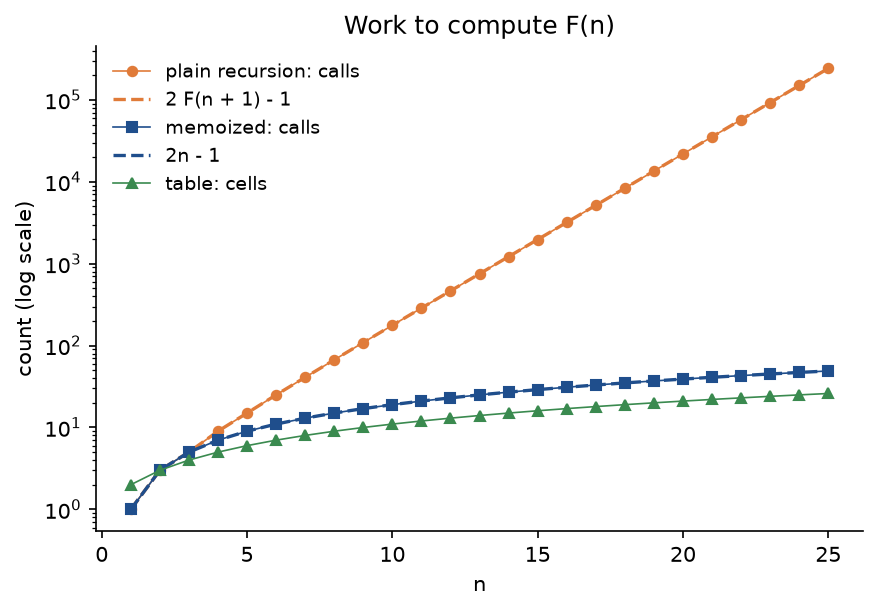
On a logarithmic axis exponential growth is a straight line: plain recursion multiplies its work by about 1.6180 for every step of n, and matches its closed form at every point. The memo and the table grow linearly and stay near the bottom of the plot.

The three tables

The cost of a table is its number of cells times the choices per cell. For rod cutting, cell j weighs j first pieces:

For the knapsack, each of the n(W + 1) cells below row 0 weighs at most two choices:

For the matrix chain, a chain of length ℓ has ℓ − 1 splits, and there are n − ℓ + 1 chains of that length:

The rod and the chain cost more per cell than the knapsack because their choices grow with the subproblem. examples/table_costs.py counts all three on random instances.

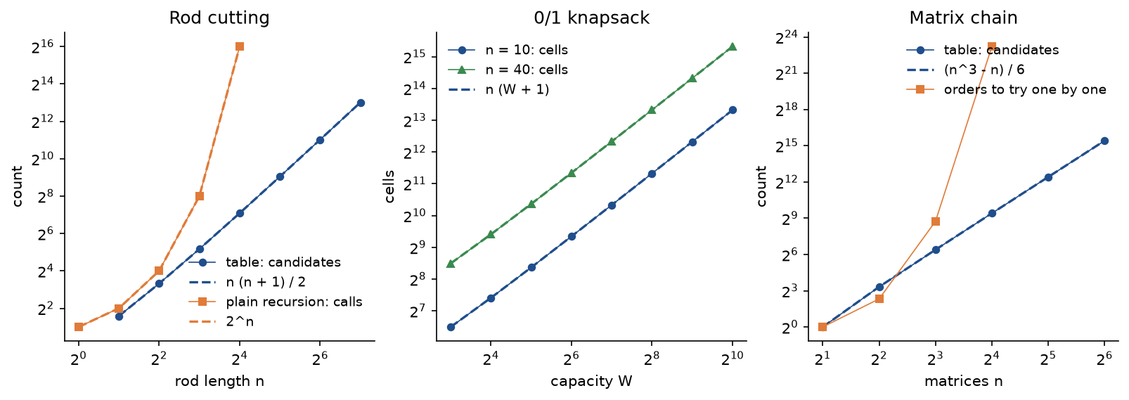
Every measured count sits on its formula. The brute-force curves show what the tables save: a rod of length 16 already needs 65536 calls without a table, and a chain of 64 matrices, which the table settles with 43680 candidates, has 94295850558771979787935384946380125 orders.

Why O(nW) is pseudo-polynomial

The knapsack table looks polynomial, Θ(nW), but W is a number in the input, and a number of b bits can be as large as 2^b:

An algorithm whose time is polynomial in the numeric values of its input but not in the length of their encoding is called pseudo-polynomial. The difference is easy to see: multiplying every weight and the capacity by 10 does not change the problem at all, adds about 3.3 bits per number, and multiplies the table by 10. The worked instance of the next section fills 36 cells; scaled by 10, 100 and 1000 it fills 324, 3204 and 32004 cells for the same answer, 42, while its input grows from 28 to 43, 59 and 75 bits.

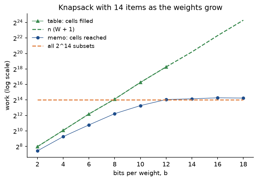
With 14 items, each extra bit per weight doubles the table, from 252 cells at 2 bits to 315126 at 12 and 20582044 at 18. The memo levels off instead, near 19449 cells, because with large distinct weights hardly any two decisions lead to the same remaining capacity, and it can never exceed the 2^(n + 1) − 1 subproblems a brute force would visit. Neither is polynomial in the input length. That is expected: the knapsack problem is NP-hard (see P and NP), so no algorithm is known that is polynomial in n and log W together. The table is still the method of choice when W is modest, and scaling the values instead of the weights turns a value-indexed version of the same table into an approximation scheme (Approximation algorithms).

What the order of a chain is worth

examples/table_costs.py also prices every order of a random chain of 9 matrices with dimensions 38, 7, 33, 50, 18, 4, 2, 11, 44 and 39.

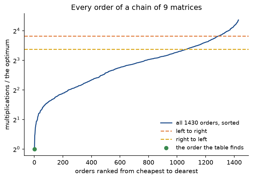
The optimum needs 13602 multiplications and the dearest of the 1430 orders 280570. Multiplying left to right, which is what a loop over the matrices does, costs 14.2004 times the optimum, and the median order 7.5249 times. On large matrices that factor is wall-clock time, which is why numerical libraries choose the order before multiplying.

Memo or table, counted

examples/fibonacci_four_ways.py measures the two costs a memo has and a table does not.

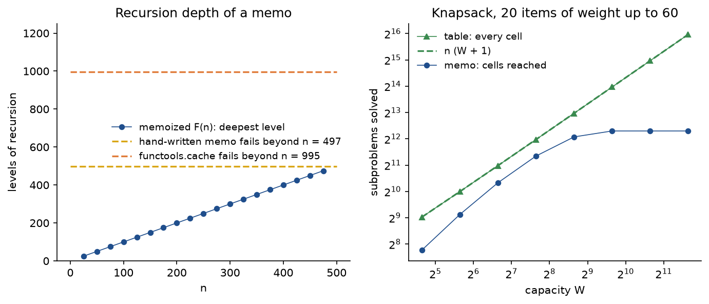
On the left, the recursion of a memoized F(n) is n levels deep, and under CPython's default limit the hand-written memo stops working beyond n = 497 and functools.cache beyond n = 995; the table computes F(100000), a number of 69424 bits, without any recursion. On the right, the memo solves between 0.4192 and 0.6468 of the knapsack table for capacities up to 400, where most capacities can be reached, but only 0.0786 at W = 3200, where the items cannot fill the bag and most cells are never asked about.

Worked example

Every step below is printed by examples/worked_example.py and asserted by tests/test_worked_example.py.

F(5) four ways

• Plain recursion makes 15 calls and 7 additions, which is 2F(6) − 1 calls and F(6) − 1 additions.
• The memo makes 9 calls, computes 6 values and answers 3 calls from the dictionary. In order: compute F(1) = 1, compute F(0) = 0, compute F(2) = 1, F(1) from the memo, compute F(3) = 2, F(2) from the memo, compute F(4) = 3, F(3) from the memo, compute F(5) = 5. The recursion first runs down the left spine to F(1), and every right child after that is a memo hit.
• The table fills [0, 1, 1, 2, 3, 5] with 4 additions.
• Two variables make the same 4 additions and keep only the last two values.

Cutting a rod of length 7

The prices of a piece of length 1 to 7 are 2, 7, 14, 17, 23, 26 and 29. The table fills r[0] = 0 and then each length, weighing every first piece i as p_i + r[j − i]:

• r[1]: cut 1 gives 2 + 0 = 2. So r[1] = 2.
• r[2]: cut 1 gives 2 + 2 = 4, cut 2 gives 7 + 0 = 7. So r[2] = 7, first piece 2.
• r[3]: 2 + 7 = 9, 7 + 2 = 9, 14 + 0 = 14. So r[3] = 14, first piece 3.
• r[4]: 2 + 14 = 16, 7 + 7 = 14, 14 + 2 = 16, 17 + 0 = 17. So r[4] = 17, first piece 4.
• r[5]: 19, 21, 21, 19 and 23 + 0 = 23. So r[5] = 23, first piece 5.
• r[6]: 25, 24, 14 + 14 = 28, 24, 25, 26. So r[6] = 28, first piece 3.
• r[7]: 30, 30, 14 + 17 = 31, 17 + 14 = 31, 30, 28, 29. Two first pieces reach 31; the shortest wins, so first piece 3.

The table is r = [0, 2, 7, 14, 17, 23, 28, 31] after 8 cells and 28 candidates, which is 7 · 8 / 2. The reconstruction cuts 3 off the 7 (first[7] = 3), then reads first[4] = 4 and cuts the rest whole: pieces 3 and 4 for 31. Plain recursion would make 2^7 = 128 calls. Greedy by price per unit length picks the piece of 3, whose 14/3 ≈ 4.6667 per unit is the best density, twice, and is left with a piece of 1 worth 2: 30 in all. The rod-cutting graph in the previous section draws the same computation as the longest path 7 → 4 → 0.

Packing a bag of capacity 8

The items are A (weight 5, value 26), B (3, 16), C (1, 13) and D (2, 3), in that order. Row 0 is all zero. Each row then copies the row above where the item does not fit and weighs leave against take where it does:

• Row A: capacities 0 to 4 copy row 0; from 5 on, taking A gives 26 + V[0][c − 5] = 26. Row: 0, 0, 0, 0, 0, 26, 26, 26, 26.
• Row B: capacities 0 to 2 copy; at 3 and 4 taking B gives 16; at 5, 6 and 7 leaving B keeps 26 against 16 for taking; at 8 taking B gives 16 + V[1][5] = 42. Row: 0, 0, 0, 16, 16, 26, 26, 26, 42.
• Row C: at 1 and 2 taking C gives 13; at 3 leaving keeps 16; at 4 taking gives 13 + V[2][3] = 29; at 5, 13 + 16 = 29 beats 26; at 6 and 7, 13 + 26 = 39; at 8 leaving keeps 42 against 13 + 26 = 39. Row: 0, 13, 13, 16, 29, 29, 39, 39, 42.
• Row D: at 0 and 1 D does not fit; everywhere else leaving D wins or ties. The ties are at capacity 3, where 3 + V[3][1] = 16 equals V[3][3] = 16, and at capacity 8, where 3 + V[3][6] = 42 equals V[3][8] = 42. Row: 0, 13, 13, 16, 29, 29, 39, 39, 42.

The table has 36 cells below row 0, 25 of them with two candidates, and the best value is V[4][8] = 42. Two different subsets reach it, and the tie at V[4][8] decides which one a backtrace reports:

• Leaving on a tie: V[4][8] = 42 equals V[3][8], so D stays out; V[3][8] = 42 equals V[2][8], so C stays out; V[2][8] = 42 differs from V[1][8] = 26, so B goes in and the room drops to 5; V[1][5] = 26 differs from 0, so A goes in. The bag holds A and B, weight 8, value 42.
• Taking on a tie: at V[4][8] taking D reaches 42, so D goes in and the room drops to 6; at V[3][6] taking C reaches 13 + 26 = 39, so C goes in and the room drops to 5; V[2][5] = 26 equals V[1][5], so B stays out; A goes in. The bag holds A, C and D, also weight 8 and value 42.

Greedy by value per unit of weight orders the items C (13 per kilogram), B (5.3333), A (5.2) and D (1.5). It takes C and B, skips A, which no longer fits in the remaining 4, takes D and stops at 32, ten short of the optimum. With items allowed to be cut, the same order takes C, B and then 4/5 of A, worth 13 + 16 + 20.8 = 49.8000, an upper bound on any whole-item answer.

Multiplying five matrices

The chain is A1 (9 by 13), A2 (13 by 6), A3 (6 by 14), A4 (14 by 5) and A5 (5 by 8), so the dimensions are 9, 13, 6, 14, 5, 8. The diagonal holds zeros. Each later cell weighs every split k as m[i][k] + m[k + 1][j] + p_(i−1) p_k p_j:

• Chains of length 2, one split each: m[1][2] = 9 · 13 · 6 = 702, m[2][3] = 13 · 6 · 14 = 1092, m[3][4] = 6 · 14 · 5 = 420, m[4][5] = 14 · 5 · 8 = 560.
• m[1][3]: k = 1 gives 0 + 1092 + 9 · 13 · 14 = 2730, k = 2 gives 702 + 0 + 9 · 6 · 14 = 1458. So 1458, split 2.
• m[2][4]: k = 2 gives 0 + 420 + 390 = 810, k = 3 gives 1092 + 0 + 910 = 2002. So 810, split 2.
• m[3][5]: k = 3 gives 0 + 560 + 672 = 1232, k = 4 gives 420 + 0 + 240 = 660. So 660, split 4.
• m[1][4]: k = 1 gives 0 + 810 + 585 = 1395, k = 2 gives 702 + 420 + 270 = 1392, k = 3 gives 1458 + 0 + 630 = 2088. So 1392, split 2, ahead of k = 1 by only 3.
• m[2][5]: k = 2 gives 0 + 660 + 624 = 1284, k = 3 gives 1092 + 560 + 1456 = 3108, k = 4 gives 810 + 0 + 520 = 1330. So 1284, split 2.
• m[1][5]: k = 1 gives 0 + 1284 + 936 = 2220, k = 2 gives 702 + 660 + 432 = 1794, k = 3 gives 1458 + 560 + 1008 = 3026, k = 4 gives 1392 + 0 + 360 = 1752. So 1752, split 4.

The table fills one diagonal per frame, 15 cells and 20 candidates in all, which is (5³ − 5)/6. The split s[1][5] = 4 says the last product is (A1 A2 A3 A4) A5; s[1][4] = 2 splits the left part as (A1 A2)(A3 A4), and s[1][2] = 1 and s[3][4] = 3 leave the two pairs as they are. The best order is (((A1 A2) (A3 A4)) A5) with 1752 multiplications: A1 A2 (702, giving a 9 by 6 matrix), A3 A4 (420, giving 6 by 5), their product (270, giving 9 by 5) and finally the 9 by 5 times the 5 by 8 (360). Multiplying left to right costs 2448 and right to left 2792; the dearest of the 14 orders costs 4298. The runner-up, ((A1 (A2 (A3 A4))) A5), costs 1755, only 3 more, because m[1][4] beat its own runner-up by the same 3: the comparison inside a cell must be done exactly, not by eye.

The code

The package dynamic_programming is plain Python, one idea per module. Importing it needs only the standard library; Matplotlib is imported by plotting.py alone, and NumPy, SciPy and NetworkX only inside the functions of comparisons.py that use them.

• counting.py holds OperationCounter, with the fields calls, hits, cells, candidates, additions, multiplications and comparisons, that every algorithm accepts as an optional counter argument, and CountedKey for library code.
• trace.py holds the Step record (action, cell name, value, the candidates weighed and the decision), record, describe and format_trace, which print the traces above.
• memo.py holds Memo, memoization written out with counts and the recursion depth.
• fibonacci.py holds the four ways and fast doubling with their closed-form counts; subproblems.py holds explore, recursion_tree_size and the Fibonacci graph.
• rod_cutting.py, knapsack.py and matrix_chain.py hold the three problems: plain recursion, memo and table, the reconstruction (reconstruct_cuts, backtrace with its tie rule, parenthesize and format_order) and the greedy rule that fails for rods.
• knapsack_variants.py holds the one-row and memoized knapsacks, brute force, the unbounded variant, the knapsack as a DAG and the scaling helpers; greedy.py holds greedy orders, the fractional knapsack and the counterexample search; chain_orders.py enumerates every order of a chain, prices it and multiplies matrices in it.
• dag.py holds WeightedDag, topological order and shortest and longest paths; line_breaking.py holds greedy and optimal line breaking for the sample project.
• invariants.py checks that every cell of a knapsack, rod or matrix-chain table satisfies its recurrence, that a selection fits and adds up, and that an evaluation order puts every subproblem after what it reads.
• workloads.py holds the worked examples and seeded random instances; drawing.py and graph_drawing.py return deterministic Graphviz text for tables, call trees and subproblem graphs.
• comparisons.py puts functools, NumPy, SciPy, NetworkX and textwrap next to the package; pitfalls.py holds deliberately broken versions for the pitfalls below; plotting.py draws every figure in the handbook's colours.

Counting and tracing never change what the code does; the text of a trace is built only when a trace list is passed. The examples run in a few seconds each from the repository root:

• examples/worked_example.py prints every step of the worked examples and writes the four generated diagram sources.
• examples/fibonacci_four_ways.py counts the four ways, finds the recursion limits and compares memo and table.
• examples/knapsack_and_greedy.py runs every greedy order against the table, measures the greedy gap on random instances and shows the pseudo-polynomial growth.
• examples/table_costs.py counts the three tables against their formulas and prices every order of a chain.
• examples/common_mistakes.py runs every broken version from pitfalls.py next to the correct code.
• examples/compare_with_libraries.py checks the package against functools, NumPy, SciPy, NetworkX and textwrap.
• examples/practice.py prints fresh exercises with their solutions; --seed gives a new set.

python algorithm-design/dynamic-programming/examples/worked_example.py
python algorithm-design/dynamic-programming/examples/fibonacci_four_ways.py
python algorithm-design/dynamic-programming/examples/knapsack_and_greedy.py
python algorithm-design/dynamic-programming/examples/table_costs.py
python algorithm-design/dynamic-programming/examples/common_mistakes.py
python algorithm-design/dynamic-programming/examples/compare_with_libraries.py
python algorithm-design/dynamic-programming/examples/practice.py --seed 7

The sample project, project/break_paragraphs.py with its helper project/book.py, sets every paragraph of a book in a column of fixed width. Greedy filling, what textwrap and most editors do, puts as many words on each line as fit, which can leave one line very loose because its next word did not quite fit. The dynamic program in line_breaking.py, in the spirit of Knuth and Plass's algorithm for TeX, chooses all the breaks of a paragraph together to minimize the sum of squared slack, the unused characters at the end of each line, with the last line free:

Squaring makes one line with 8 spare characters cost more than two lines with 4 each. Subproblem: best(j), the least cost of setting the first j words; choice: where the last line starts.

It is a shortest path from word boundary 0 to word boundary n in the DAG whose edges are feasible lines (line_dag). For each end the loop walks the start backwards only while the line still fits, so the work is the number of feasible lines, about n times the number of words a line holds:

The text is Household Tales by the Brothers Grimm in Margaret Hunt's translation. Its opening paragraph, "In old times when wishing still helped one", from The Frog-King, is the paragraph Knuth and Plass set to demonstrate their algorithm, there in a slightly different wording. The project downloads it once from Project Gutenberg (ebook 5314) into .data/dynamic-programming/ and checks the text between Gutenberg's start and end markers against a pinned SHA-256 digest. The default run sets the 1648 paragraphs of the 200 tales, 277129 words with a mean length of 4.1829 characters, at a width of 40 characters, prints the opening paragraph both ways, and finishes in about 2 seconds. Options --width, --tales, --min-words and --show change the setup, --synthetic uses generated words instead of the book, --no-verify accepts a changed download, and --figures writes the PNGs elsewhere.

python algorithm-design/dynamic-programming/project/break_paragraphs.py
python algorithm-design/dynamic-programming/project/break_paragraphs.py --width 60

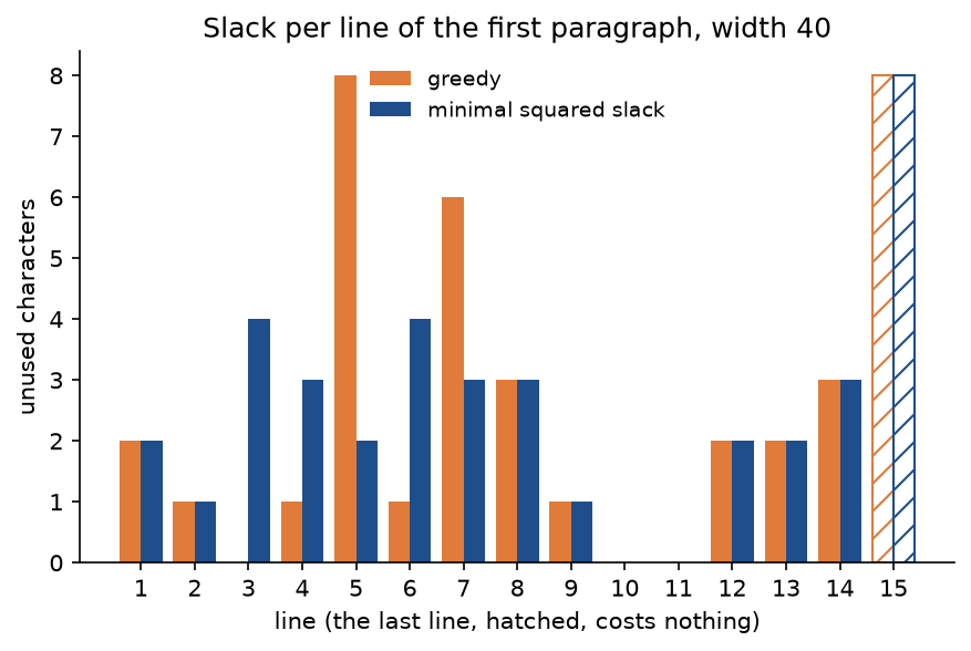
Both settings use 15 lines. The greedy one has two gaping lines, 8 and 6 characters short, and a total squared slack of 134; the dynamic program moves a word or two between lines 3 to 7 and gets 86, with no line more than 4 characters short. Over the whole book greedy filling is identical to textwrap's on all 1648 paragraphs, and the dynamic program cuts the total squared slack from 402806 to 333819, 0.1713 less, improves 1042 of the paragraphs, lowers the mean loosest line of a paragraph from 6.6569 to 5.3431 characters, and needs only 2 more lines than greedy's 38025 in the whole book.

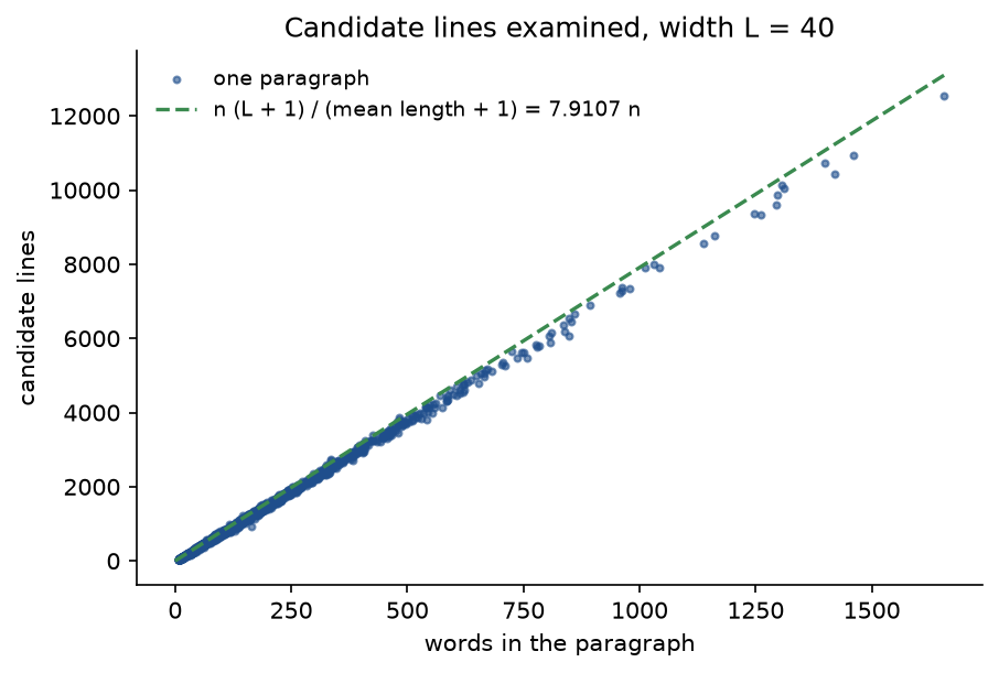
The work is linear in the paragraph: 2060574 candidate lines for 277129 words, 7.4354 per word against the predicted 7.9107, which slightly overestimates because the words near the start of a paragraph have fewer possible line starts and a line rarely fills to its last character. A naive search over all 2^(n − 1) ways to break a paragraph of n words would be hopeless for a single paragraph of a few hundred words; the table needs one cell per word boundary, 278777 in all.

The notebook dynamic_programming.ipynb follows this page: the four Fibonacci programs counted, the subproblem graph, every worked table filled step by step, the tie rules, greedy against the knapsack, memo against table, the DAG view and the project on a few tales. The tests in tests check the worked examples value by value, every table against its recurrence on random instances, the closed-form counts, the agreement with brute force, NumPy, SciPy, NetworkX and textwrap, and every broken version in pitfalls.py, and run in a few seconds:

python -m pytest algorithm-design/dynamic-programming

All data except the book are synthetic, generated from seeds by workloads.py. The book is Household Tales by Jacob and Wilhelm Grimm, translated by Margaret Hunt (1884), Project Gutenberg ebook 5314, public domain in the United States; the file is distributed under the Project Gutenberg License, downloaded at runtime and never committed.

In practice

functools.cache and lru_cache

In Python, memoization is one decorator. functools.cache (an unbounded lru_cache) keeps a dictionary keyed by the arguments, so they must be hashable: a list argument raises TypeError, and a tuple or an index works. cache_info() reports hits and misses, which match the hand-written Memo exactly, and the C implementation is roughly ten times faster in wall-clock time, as compare_with_libraries.py prints for F(400). It also reaches about twice the recursion depth, since it adds no Python frame. A bounded lru_cache(maxsize=k) evicts the least recently used entries, which can bring the exponential recursion back: F(30) needs 31 misses with an unbounded cache or with three entries, 41641 misses with two, and with one entry the misses of F(20), 21891, equal the calls of plain recursion. A cache attached to a function also lives as long as the function, so a module-level cached function fed many different instances keeps all their answers alive; create the cached function inside the solver, as fib_cached does, or call cache_clear().

NumPy's multi_dot

numpy.linalg.multi_dot multiplies a chain of arrays in the cheapest order. For more than three arrays it computes the split table with the same recurrence as matrix_chain_order, and compare_with_libraries.py shows its split table equal to ours on 50 random chains of 10 matrices. The example also multiplies the worked chain in all 14 orders and a chain of 8 matrices in all 429 orders with NumPy and finds every product exactly equal to multi_dot's, which is associativity at work: the order changes the cost, never the result (exactly so for integers; in floating point the results agree to rounding). When matrices of very different shapes meet, such as a matrix times a matrix times a vector, the order is worth a factor of the matrix size, and A @ B @ v written in Python evaluates left to right.

Integer programming for the knapsack

SciPy has no knapsack routine, but scipy.optimize.milp solves the knapsack as an integer linear program with the HiGHS solver, which uses branch and bound with linear-programming bounds rather than a table. scipy_knapsack agrees with the table on all 30 random instances of 30 items with capacity 700, and at that size the pure-Python table and the solver take about as long. The solver's running time does not depend on the magnitude of the weights, so it wins as W grows; the table wins for small integer capacities, many repeated instances, or when every capacity's answer is wanted at once. Dedicated codes such as Pisinger's combine both ideas and solve instances with thousands of items.

Elsewhere

NetworkX's dag_longest_path_length returns 31 on the rod-cutting graph and 42 on the knapsack graph, the same longest paths as dag_longest_paths. textwrap's lines equal break_greedy's on every paragraph of the book, while TeX and the paragraph composers of desktop publishing programs choose breaks for a whole paragraph at once, in the spirit of the project's dynamic program, and CSS now lets browsers improve on greedy breaking with text-wrap: pretty. Dynamic programming runs much of the software around you: diff and version control align files with longest common subsequences, spell checkers and DNA aligners use edit distance (both on Dynamic programming on sequences), speech recognizers and GPS map matching use the Viterbi algorithm, routers use Bellman-Ford, Floyd-Warshall fills a table of all pairs (see All-pairs shortest paths), query optimizers in databases choose join orders much as the matrix chain chooses product orders, and reinforcement learning is built on Bellman's equation. When to use which:

• Use functools.cache on a recursive function when the recurrence is natural, the depth stays well below the recursion limit and only some subproblems matter.
• Use an explicit table when every subproblem is needed, when the depth could be large, or when rolling rows saves the memory you need.
• Use a library solver (an integer programming solver for knapsack-like problems, NetworkX for paths) when the problem fits its model and the numbers are too large for a table.
• Use a greedy rule only with a proof such as the exchange argument; otherwise check it against the table on small instances, as the tests here do.

Pitfalls

• Defining the subproblem too narrowly. A knapsack memo keyed on the remaining capacity alone, without the number of items still to decide, answers different questions with the same entry: on four items of weight 1 worth 5, 8, 3 and 6 with capacity 3 it returns 13 instead of 19. The key must include everything the future depends on. examples/common_mistakes.py runs this and every following mistake.
• Writing the fit test as w < c. An item that exactly fills the remaining room fits; with w < c an item of weight 5 is never put into a bag of 5, and the answer 12 becomes 10.
• Filling the table in an order that reads empty cells. Filling the matrix-chain table row by row from the top reads cells below that are still zero and reports 936 for the worked chain instead of 1752. Fill by chain length, or rows from the bottom up; check any order with check_evaluation_order.
• Visiting the capacities upwards in a one-row knapsack. The cell for c then reads a value that already includes the current item, so each item can be taken many times: the worked items give 104 instead of 42. Go from W down to w_i.
• Reconstructing without lowering the remaining capacity. After taking an item, the backtrace must continue from column c − w_i; staying in column c reports items that overflow the bag. When tracing by hand, write the remaining capacity next to every step.
• Comparing backtraces without a tie rule. When V[i][c] equals both V[i − 1][c] and v_i + V[i − 1][c − w_i], both subsets are optimal; say which rule you use, as the worked example's two answers, A and B against A, C and D, show.
• Forgetting a choice in the recurrence. A rod recurrence over the cuts 1 to n − 1 forgets to sell the rod uncut: prices 1 for a piece of 1 and 10 for a piece of 3 give 3 instead of 10 for a rod of 3.
• Mixing 0-based dimension lists with 1-based matrix names. Ai is p[i − 1] by p[i], so the cost of the last product is p[i − 1] p[k] p[j]; writing p[i] p[k] p[j] gives 2289 for the worked chain instead of 1752. A chain of n matrices has n + 1 dimensions.
• Trusting greedy for whole items. Value per weight is optimal only when items can be cut; on the worked items it gets 32 against 42, and on the trap family its share of the optimum tends to zero.
• Memoizing with a mutable default argument. def solve(n, memo={}) creates the dictionary once, so a second instance is answered from the first one's entries: the rod with the worked prices is reported to earn 16 instead of 31 after a call with other prices.
• Memoizing on unhashable arguments. functools.cache raises TypeError for a list; pass a tuple or an index into a list held outside.
• Recursing past the limit. A memoized F(2000) raises RecursionError while two variables compute it at once. Prefer a table for long chains of subproblems, and do not raise the recursion limit in library code.
• Calling a pseudo-polynomial table polynomial. Θ(nW) is exponential in the number of digits of W; scaling the weights by 1000 multiplies the work by 1000 for the same answer.
• Mixing Fibonacci conventions. With F(1) = 0 and F(2) = 1 every value is shifted by one index; compare F(10) = 55 in this page's convention before comparing anything else.

Further reading

• R. Bellman, "The theory of dynamic programming", Bulletin of the American Mathematical Society 60(6), 503-515, 1954, and Dynamic Programming, Princeton University Press, 1957. The method, its name and the principle of optimality.
• D. Michie, "Memo functions and machine learning", Nature 218, 19-22, 1968. The origin of the word memoization.
• T. H. Cormen, C. E. Leiserson, R. L. Rivest and C. Stein, Introduction to Algorithms, fourth edition, chapter 14, MIT Press, 2022. Rod cutting, matrix-chain multiplication and the elements of dynamic programming.
• S. Dasgupta, C. H. Papadimitriou and U. V. Vazirani, Algorithms, chapter 6, McGraw-Hill, 2006. Dynamic programming presented as shortest paths in a DAG, the knapsack and chain matrix multiplication.
• J. Kleinberg and É. Tardos, Algorithm Design, chapter 6, Addison-Wesley, 2005. Weighted interval scheduling, segmented least squares and the knapsack, with careful correctness proofs.
• J. Erickson, Algorithms, chapter 3, 2019, freely available online. Recursion, memoization and dynamic programming with many exercises.
• G. B. Dantzig, "Discrete-variable extremum problems", Operations Research 5(2), 266-288, 1957. The knapsack problem and the greedy solution of its fractional version.
• H. Kellerer, U. Pferschy and D. Pisinger, Knapsack Problems, Springer, 2004. Pseudo-polynomial algorithms, approximation schemes and practical solvers.
• S. S. Godbole, "On efficient computation of matrix chain products", IEEE Transactions on Computers C-22(9), 864-866, 1973. The cubic dynamic program for matrix chains.
• T. C. Hu and M. T. Shing, "Computation of matrix chain products", parts I and II, SIAM Journal on Computing 11(2), 362-373, 1982, and 13(2), 228-251, 1984. An O(n log n) algorithm for the same problem.
• D. E. Knuth and M. F. Plass, "Breaking paragraphs into lines", Software: Practice and Experience 11(11), 1119-1184, 1981. Optimal line breaking in TeX, the model for the sample project.
• The Python documentation of functools.cache and functools.lru_cache, and the NumPy documentation of numpy.linalg.multi_dot.