AVL trees

A binary search tree answers lookups, insertions, deletions and ordered questions such as "the largest key below x" along one path from the root, so it is exactly as fast as it is short. Left to itself it is not short: keys that arrive in increasing order, the most common order in practice (timestamps, counters, sorted files), turn it into a path as long as the input. The AVL tree, published by Adelson-Velsky and Landis in 1962 and the first balanced search tree, fixes that with one local rule: at every node the two subtrees differ in height by at most one. This page recaps search trees, defines heights and balance factors with one stated convention, derives the height bound of 1.4405 log2(n + 2) from the sparsest AVL trees and the Fibonacci numbers, works through the four imbalance cases and the rotations that repair them, traces insertion and deletion rotation by rotation, compares storing heights with storing balance factors, measures heights and rotations against a plain search tree, and checks everything against sortedcontainers. Afterwards you will be able to insert into and delete from an AVL tree by hand naming every repair, implement and test one yourself, and decide when a balanced tree, a red-black tree or a library sorted container is the right tool. It builds on Binary search trees and uses the counting of Asymptotic analysis and the recurrences of Recurrences.

The structures need only the standard library; to run the plots and the notebook install the base group, and the structures group for the comparison with sortedcontainers.

Intuition

Think of a hanging mobile: every bar holds a left arm and a right arm, and every arm holds either a weight or another bar. A mobile hangs well if no bar tilts much. Hang new weights wherever they belong and, sooner or later, one arm grows far heavier than its partner and the whole thing leans. Rebalancing the entire mobile after each new weight would be absurd. The AVL rule is the sensible compromise: every bar may tilt by one notch, never by two. When a new weight makes some bar tilt by two, you rehang three pieces right at that bar, which straightens it without disturbing anything above or beside it.

In a search tree the bars are nodes, the weight of an arm is the height of a subtree, and rehanging three pieces is a rotation. The payoff is that no root-to-leaf path is much longer than in a perfectly balanced tree, whatever order the keys arrive in.

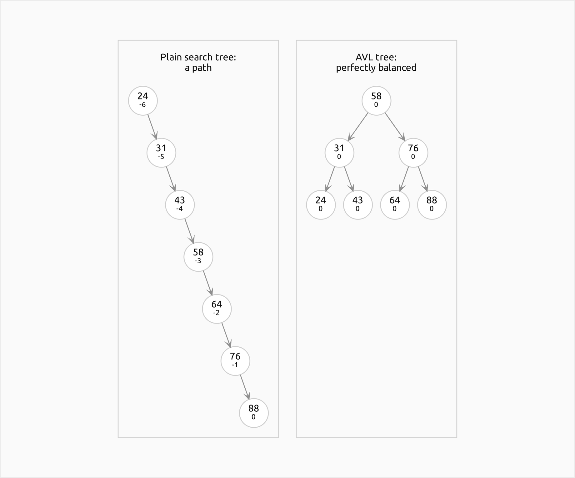
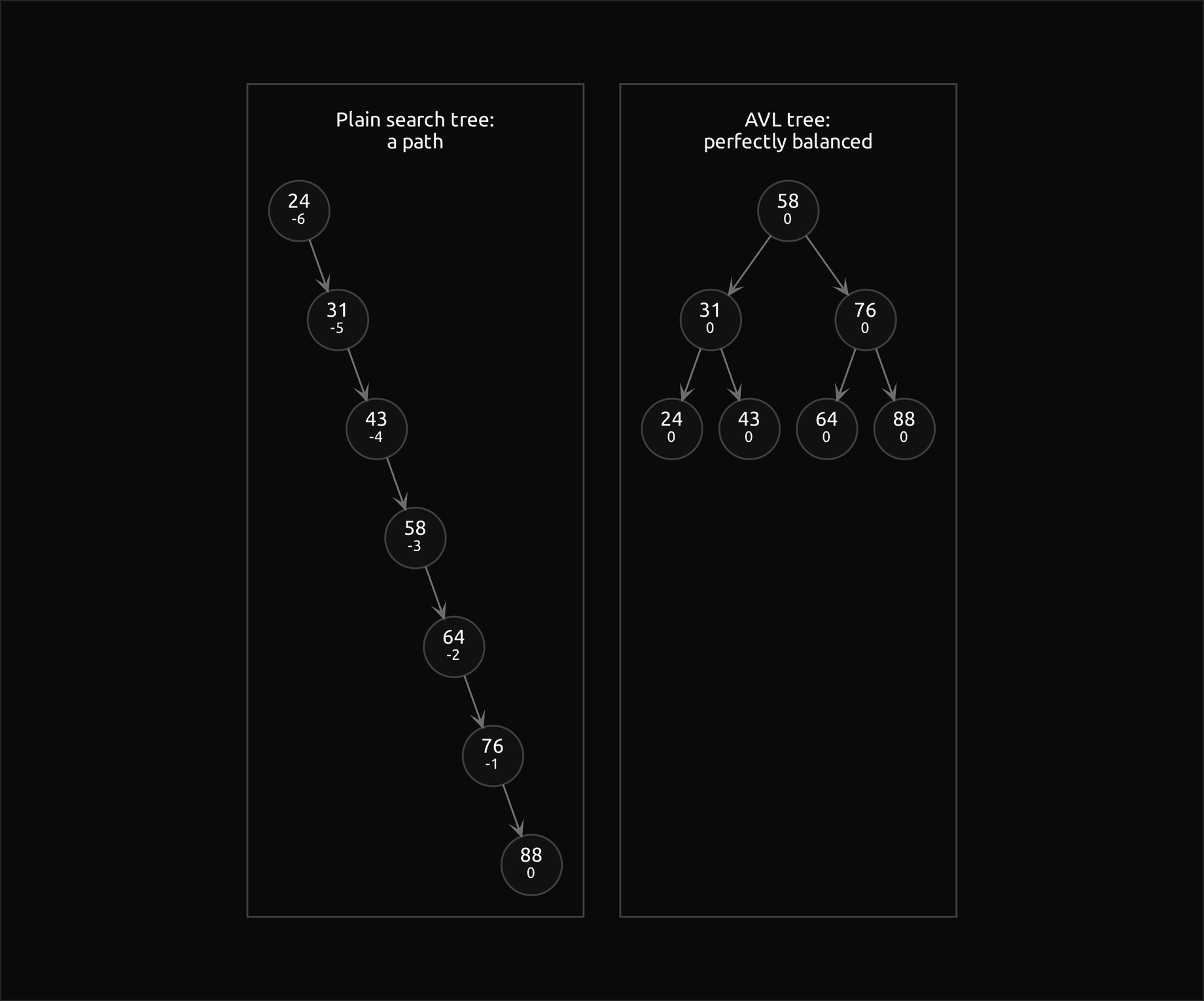
Every node shows its key and, under it, its balance factor. The plain tree on the left spends seven comparisons to find 88; the AVL tree on the right never needs more than three, and it got there with four rotations made while the keys arrived.

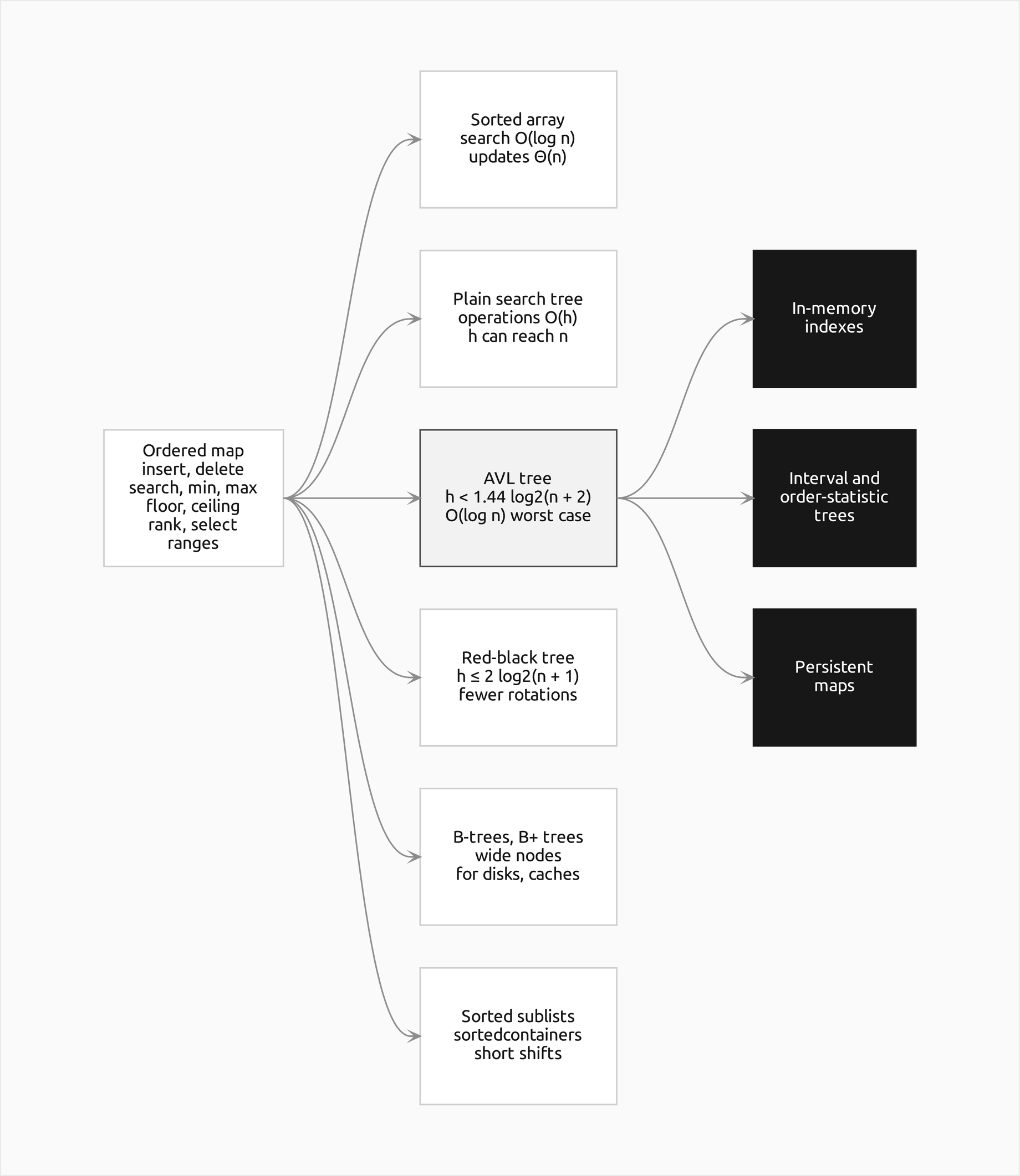
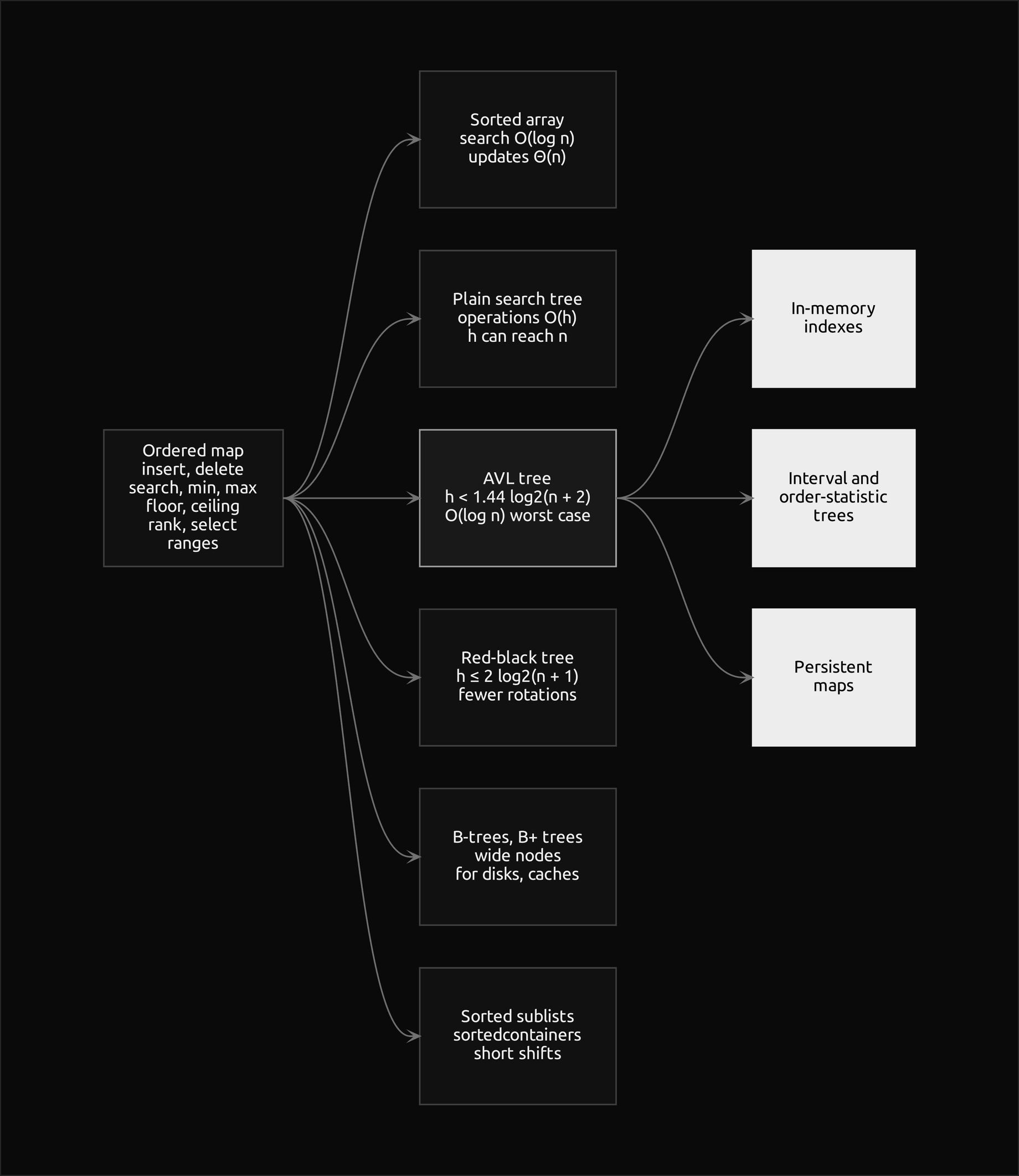
The AVL tree, the highlighted box in the middle column, is one of several ways to implement an ordered map. A hash table answers "is x present?" faster, but only an ordered structure answers "what comes after x?", "how many keys lie between a and b?" or "which key is the tenth smallest?".

How it works

Binary search trees in brief

A binary search tree stores one key per node, and every node has a left and a right subtree, either of which may be empty. The search-tree property orders a node against its whole subtrees, not just its children:

So an in-order walk (left subtree, node, right subtree) lists the keys in increasing order. Keys are distinct; inserting a key that is already present replaces its value.

• Search compares the key with the root: smaller goes left, larger goes right, equal is found, and an empty subtree means absent. The property guarantees that a present key lies on this one path. In the tree built from 47, 24, 73, 29, 61, 88, 21 and 38, searching for 38 compares with 47, 24, 29 and 38: four comparisons.
• Insertion is a search that fails, followed by hanging a new leaf where the search fell off the tree. Inserting 33 into that tree passes 47, 24, 29 and 38 and becomes the left child of 38. Nothing else moves, which is why the order is kept, and also why the tree's shape depends entirely on the order of insertions.
• Deletion has three cases. A leaf is cut off. A node with one child is replaced by that child. A node with two children takes the key of a donor, its in-order successor (the leftmost node of its right subtree) or its in-order predecessor (the rightmost node of its left subtree); the donor has at most one child and is removed by one of the first two cases. Deleting 47 from the tree above with the successor rule moves 61 into the root.

Every one of these costs one comparison per level on one path, and a tree of height h has h + 1 levels, so a search tree of height h does each operation in O(h):

The height is the whole story. A random insertion order gives an expected height that grows like 2.99 log2 n for very large n (about 33 for 16384 keys in the measurements below), but sorted, reverse sorted or alternating (smallest, largest, second smallest, ...) orders give a height of n − 1, and every operation becomes a linear scan. The package's BinarySearchTree is this plain tree, written without recursion so that such paths cannot overflow Python's stack.

Height and the balance factor

This page counts height in edges, as the rest of the handbook does: a leaf has height 0, an empty subtree height −1, and a node one more than its taller subtree. The height of a tree is the number of edges on its longest root-to-leaf path, one less than the number of keys on that path, so a search makes at most h + 1 comparisons.

The balance factor of a node is the height of its left subtree minus the height of its right subtree:

A positive factor means the node leans left, a negative one that it leans right. An AVL tree is a search tree in which every node has a factor of −1, 0 or +1:

Books differ on both conventions, and mixing them is the most common source of wrong answers. Some count height in nodes (a leaf at 1, an empty subtree at 0); that raises every height by one, changes no balance factor, and turns the bound derived below into h < 1.4405 log2(n + 2) − 0.3277, the form many books quote. More dangerously, many define the factor the other way round, right height minus left height, so that the same left-leaning node is +1 in one book and −1 in another. Rule tables for choosing rotations are written for one sign, and applied with the other they choose the wrong rotation. Pick one convention, write it down, and translate every table you borrow; this page and the package use left minus right throughout.

Each node of the package's Node stores its height and also its size, the number of keys in its subtree, which the ordered queries below need. Both are recomputed from the children by update(node), which therefore must always run on a child before its parent.

Rotations

A rotation is a local change of three links that moves one node up a level and another down, while keeping the keys in order. A right rotation at z lifts its left child y into z's place: z becomes y's right child, and y's old right subtree B, whose keys lie between y and z, becomes z's left subtree. In both trees the in-order walk is the same:

A left rotation is the mirror image. A rotation costs O(1): three pointers change, and the heights and sizes of the two nodes that moved are recomputed, the lower one (z) first, because the upper one's height is computed from it. Everything inside A, B and C is untouched, so their heights do not change.

The four imbalance cases

Suppose some node z has reached a factor of +2 or −2. Call the child of z on its taller side y, and the child of y on the path that made it tall x. The four ways the path can go give the four cases:

• Left-left: z is +2 and y leans left (or is level). One right rotation at z.
• Right-right: z is −2 and y leans right (or is level). One left rotation at z.
• Left-right: z is +2 but y leans right, towards x. First a left rotation at y, which turns the shape into left-left, then a right rotation at z. Together they lift x above both y and z.
• Right-left: the mirror image, a right rotation at y and then a left rotation at z.

The first two are outside cases, where the tall part lies on the outer edge of z's subtree, and a single rotation moves it up. The other two are inside cases, where the tall part sits in the middle; a single rotation would only move it to the other side, and two rotations are needed. The package decides with classify(z), which reads only the factors of z and y, and plan(z) lists the rotations.

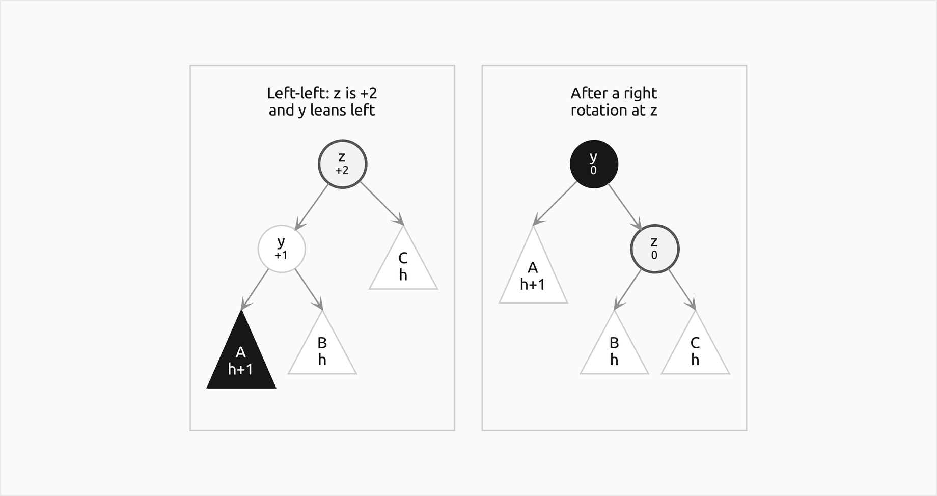
The triangles stand for whole subtrees with their heights relative to some h. In the first frame the filled triangle is the subtree an insertion made taller, z is outlined in every frame as the node being repaired, and in the second frame the filled node y is the one that moved up. After the rotation, y and z are level and the subtree is exactly as tall as it was before the insertion:

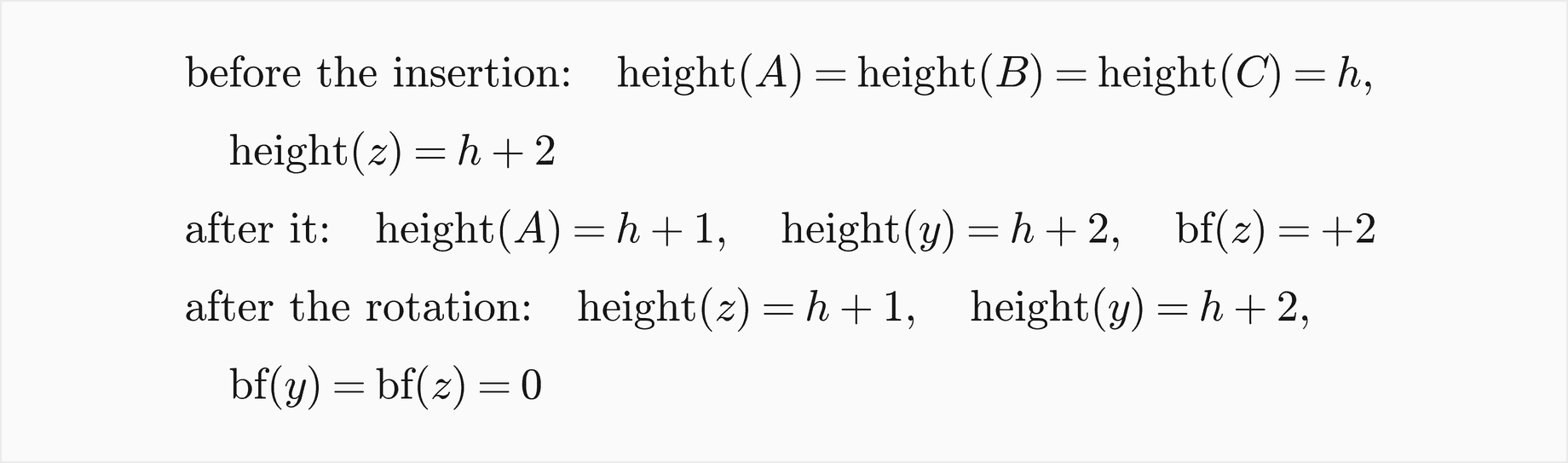
The subtree had height h + 2 before the insertion and has height h + 2 after the repair, so no node above it sees any change.

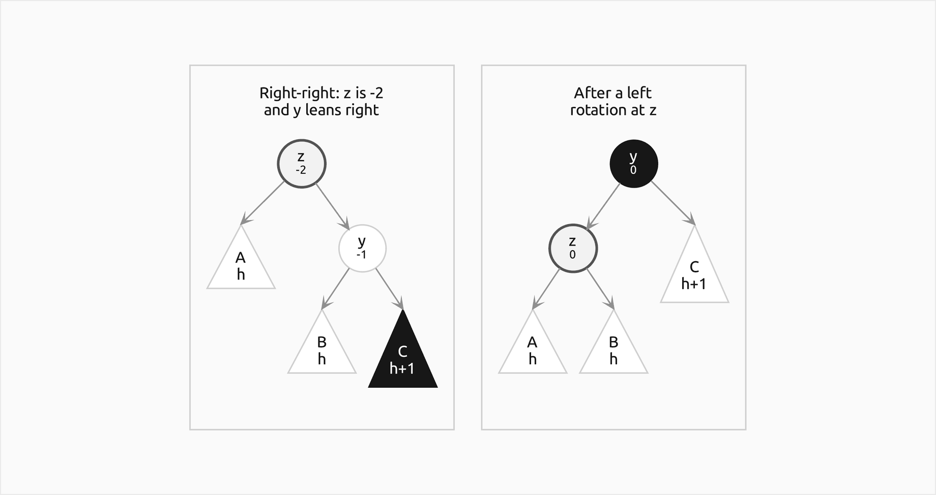
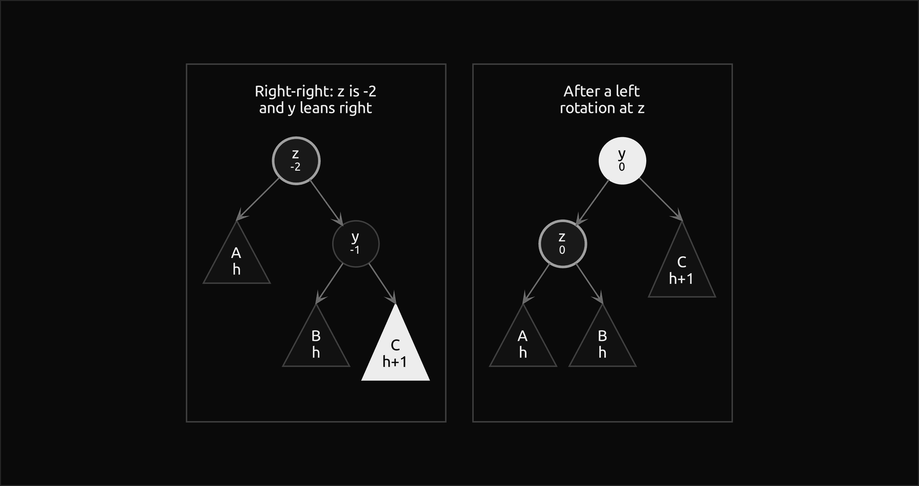
The right-right case is the same picture reflected, repaired by a left rotation.

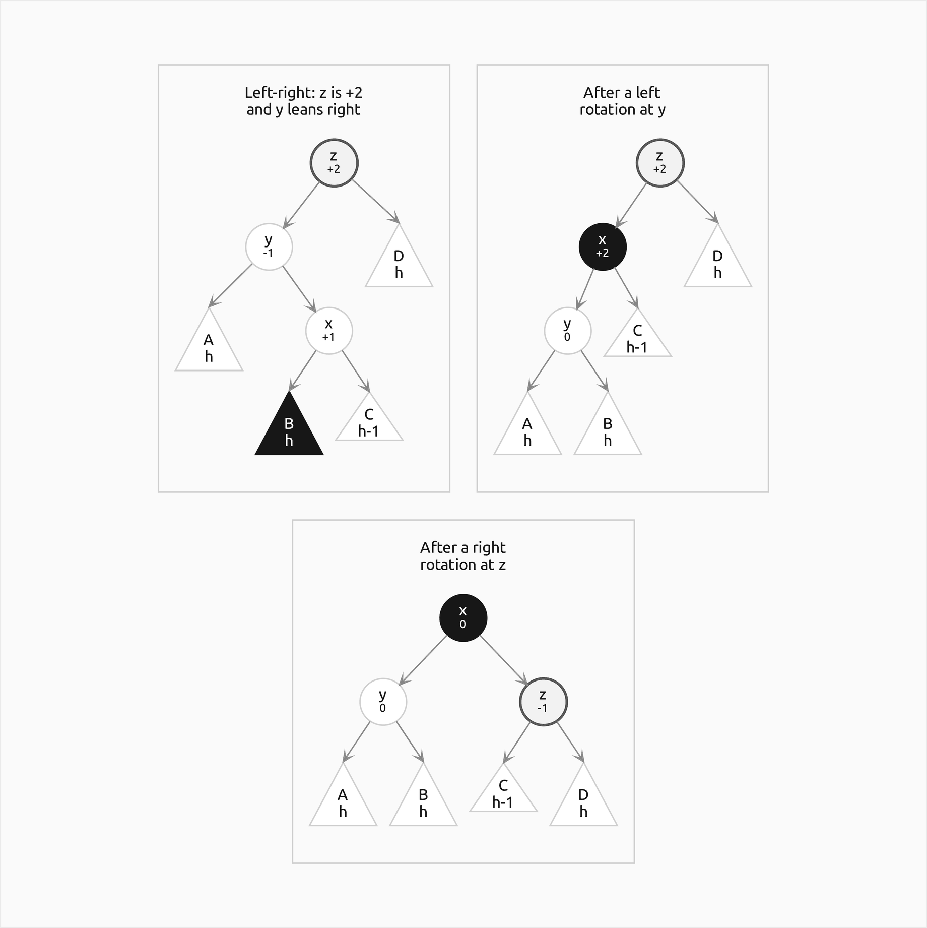
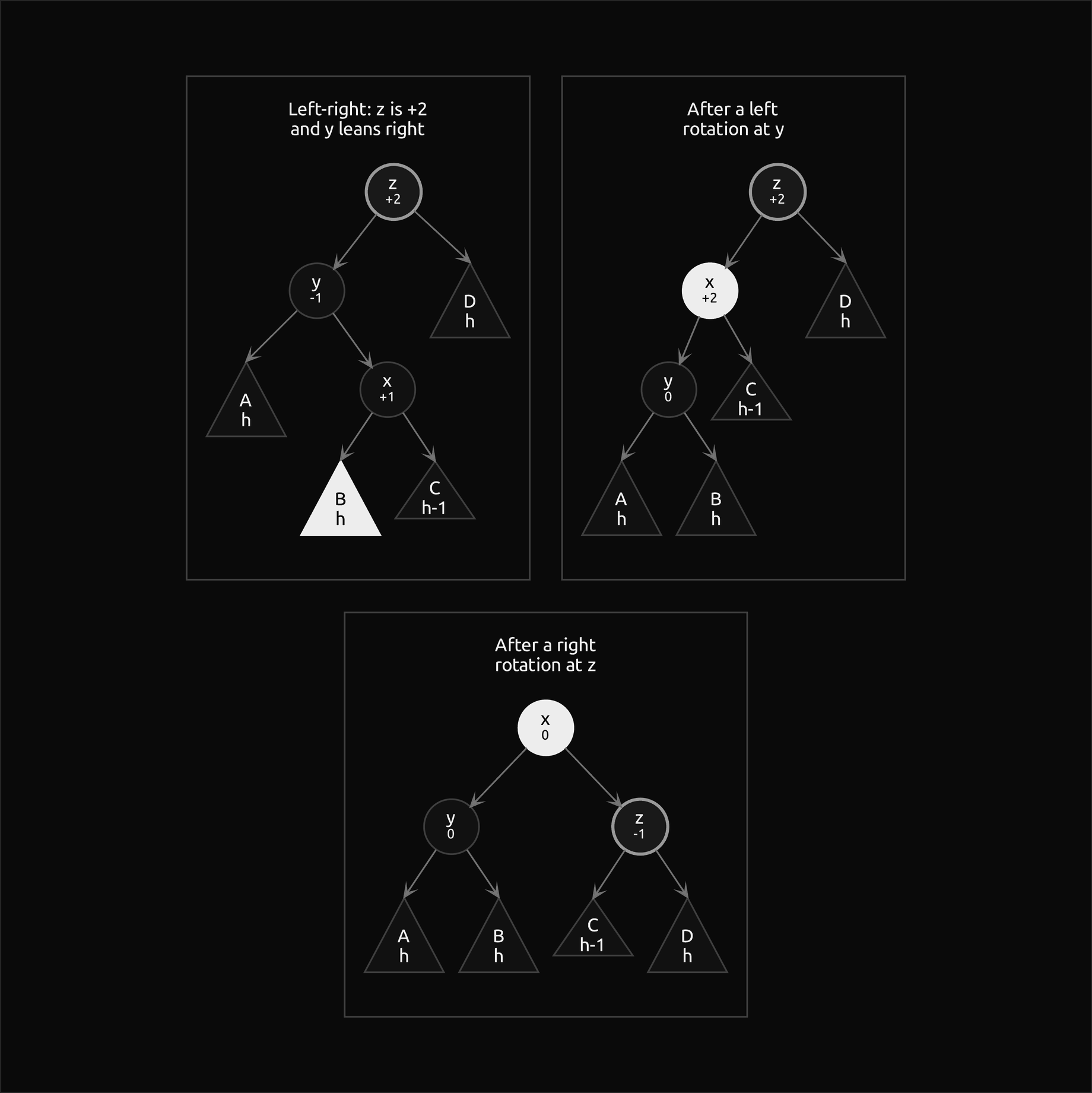
The second frame, top right, is not yet balanced: x is at +2 there, because the first rotation only turned the inside case into an outside one. After the second rotation x is the root and level, and y and z share its old children between them. Which of y and z ends up level depends on which of B and C was the taller, but the height is again the old one:

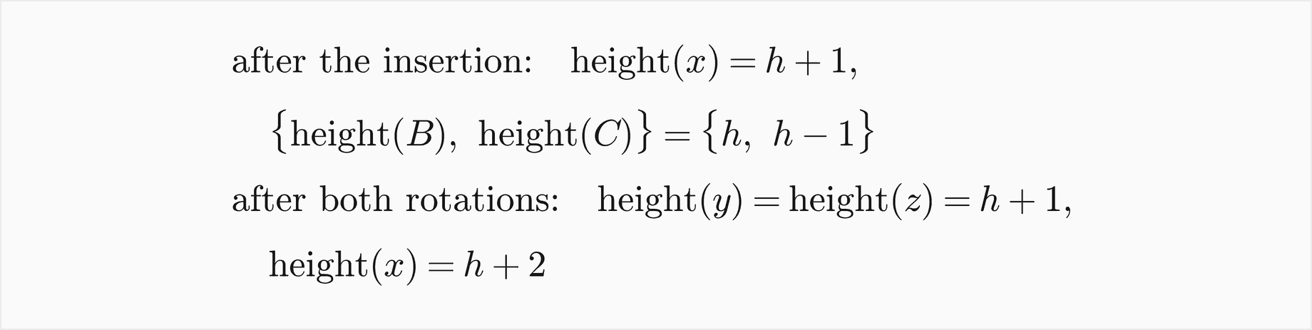
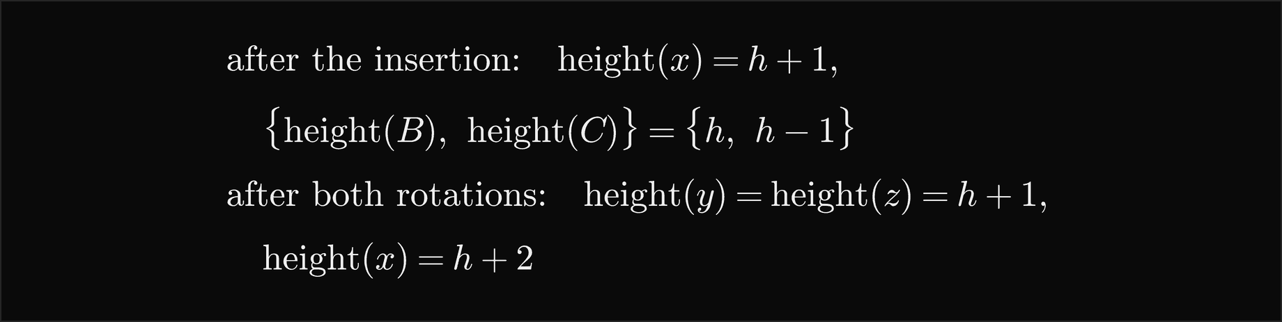
Again the repaired subtree has the height h + 2 it had before the insertion.

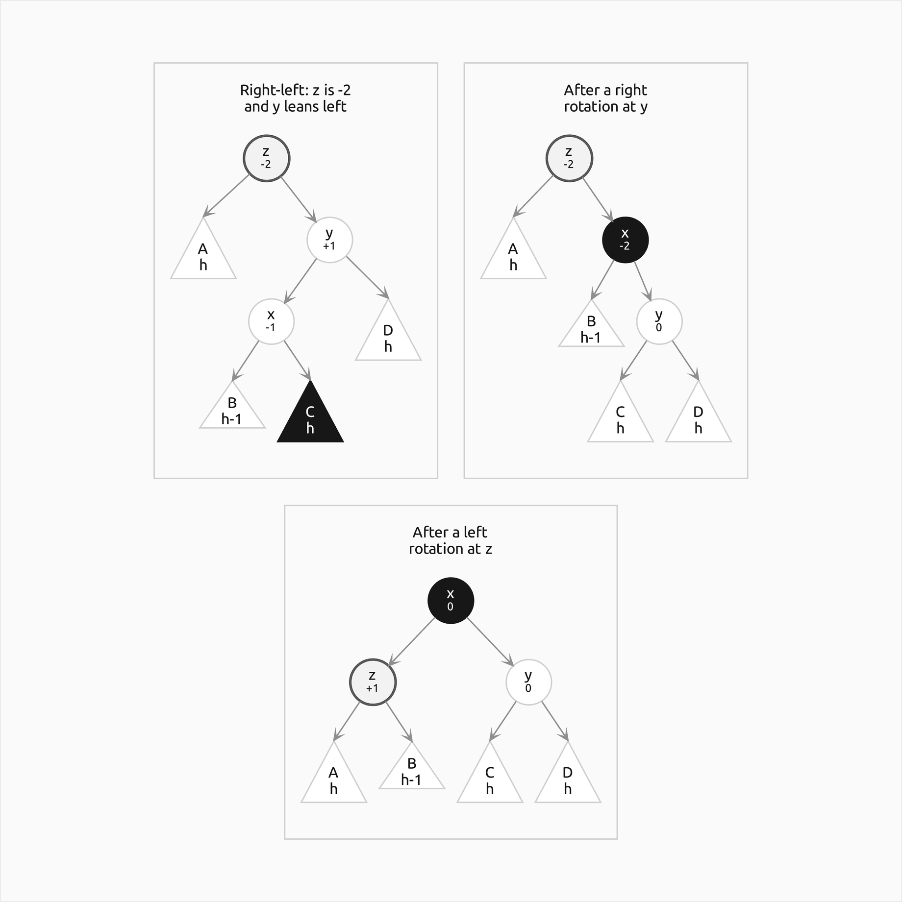
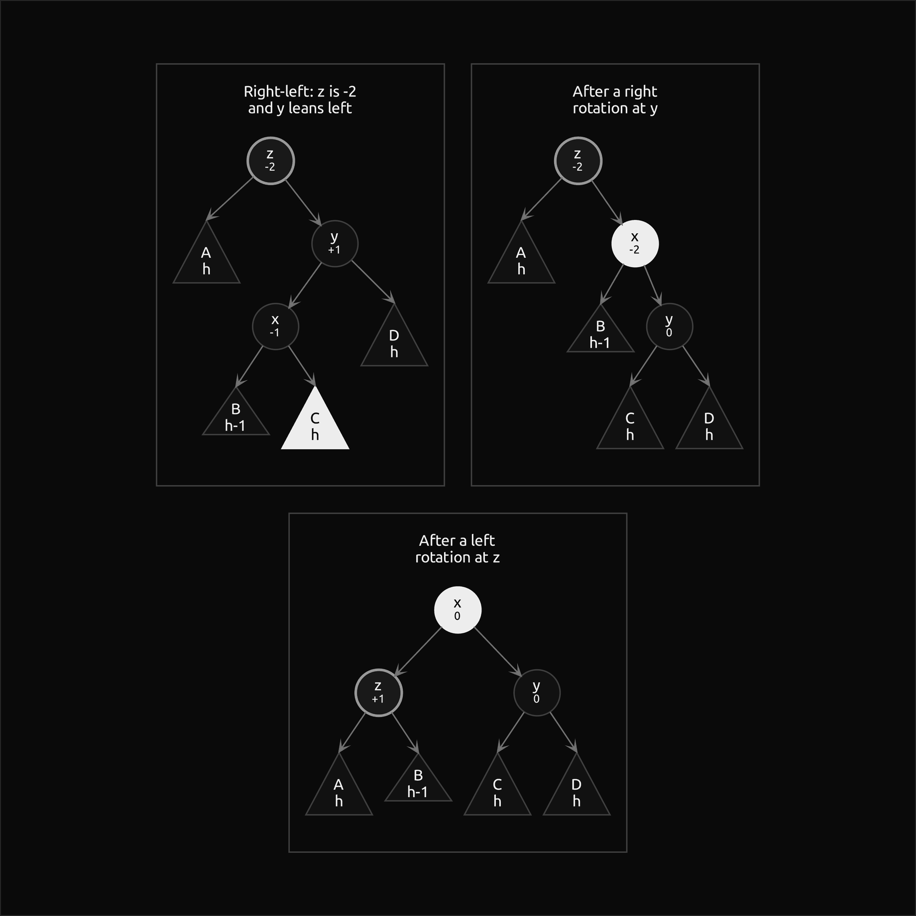
The right-left case mirrors left-right: right rotation at y, left rotation at z, x on top.

Insertion

Insertion is a search-tree insertion followed by retracing:

1. Search for the key, remembering the path. If it is found, replace its value and stop.
2. Hang a new leaf, of height 0 and factor 0, where the search fell off the tree.
3. Walk back up the path. At each node recompute the height and the factor. If the factor is +2 or −2, repair that node with the rotations of its case.
4. As soon as some subtree on the path has the same height it had before the insertion, nothing above it can change height or balance, and the walk can stop.

Only nodes on the path can change, because only their subtrees gained a node. The first node found unbalanced is the lowest one, and repairing it ends all balance work: the formulas above show that after either repair the subtree is back at the height it had before the insertion, so every ancestor sees exactly the heights it saw before and keeps its old, valid factor. An insertion therefore makes at most one repair, a single or a double rotation. Repairing a higher unbalanced node instead of the lowest one does not work, because the lower one stays unbalanced. The package's retrace keeps walking to the root after the heights stop changing only to add one to the sizes on the path; a tree without sizes would stop there.

Deletion

Deletion is a search-tree deletion followed by the same retracing, starting from the parent of the node that was physically removed. For a node with two children that is the donor's old parent, often several levels below the node whose key was named; starting the walk at the named node leaves stale heights below it.

Removing a node can only make subtrees on the path shorter. At each node of the walk there are three outcomes:

• The node was level and now leans by one away from the shorter side. Its height did not change, and the walk stops.
• The node leaned towards the shorter side and is now level. It lost one level of height, and the walk continues.
• The node leaned away from the shorter side and is now at +2 or −2. It is repaired, by the same four cases, with y the child on the taller side, which is the side the deletion did not touch.

Here deletion differs from insertion. If y is level, a case insertion never produces, the single rotation is the correct repair and leaves the subtree at its old height, and the walk stops. If y leans either way, the repair leaves the subtree one level lower than it was, so its parent may now be unbalanced too, and the walk continues:

A single deletion can therefore repair nodes at many levels. The cost section shows that it repairs at most one node in every two levels and that the sparsest AVL trees reach that limit. Some books name the deletion repairs after the side that lost height and the factor of y: R0, R1 and R−1 when the right side shrank, L0, L1 and L−1 when the left side shrank. The numbers are balance factors, so their meaning depends on the sign convention. With left minus right, R0 and R1 are left-left repairs, R−1 is left-right, L0 and L−1 are right-right and L1 is right-left; R0 and L0 keep the height. With right minus left, the 1 and −1 swap, which is how rule tables from different sources end up contradicting each other. A rule that does not depend on signs is safer: if the taller child of the unbalanced node leans the same way as the node or is level, rotate once; if it leans the other way, rotate twice.

Ordered queries, ranks and sizes

Because the keys are in search-tree order, an AVL tree answers more than membership, each along one path:

• floor(x), the largest key at most x: search for x, remembering the last node where the search turned right.
• ceiling(x), the smallest key at least x: the mirror image.
• min and max: the ends of the leftmost and rightmost paths.
• rank(x), the number of keys smaller than x, and select(i), the key of rank i: these need the subtree sizes each node stores. Turning right past a node skips its left subtree and the node itself.
• range(low, high), the keys with low ≤ key < high in order: an in-order walk that never enters a subtree lying wholly below low and stops at the first key at least high.

Keeping a size in each node is the simplest augmentation of a balanced tree: a rotation changes the sizes of exactly the two nodes whose heights it recomputes, and in the same order. Augmented trees develops the general rule. A range query that reports k keys visits the search path for low, the k reported nodes, and the nodes still waiting on its stack at the end, which lie on one root-to-leaf path; each path has at most h + 1 nodes:

The counter's visits field counts those nodes, and the tests and the sample project check the bound on thousands of queries.

Storing heights or balance factors

The original AVL tree stored only each node's balance factor, which takes two bits, instead of its height, which for a billion keys still takes six. Retracing then works on factors directly: after an insertion the parent's factor moves by one towards the side that grew, and the walk stops when it becomes 0 or after a repair; after a deletion it moves away from the side that shrank, and the walk stops when it becomes ±1 or when a repair leaves the new subtree root leaning. A rotation must compute the new factors from the old ones. Writing p and q for the heights of y's subtrees and r for the height of z's other subtree in a right rotation at z:

These two updates, with their mirror images for left rotations, hold for every case after insertions and deletions alike. BalanceFactorTree implements this representation; it makes exactly the same rotations as the height-storing AVLTree and builds exactly the same shapes, which the tests and an example check after every operation. Heights are easier to get right, because each node's state is recomputed from its children rather than updated by a rule, and they are what most modern implementations store; factors save memory in languages where two bits can be packed into a pointer, and they let retracing stop without reading any sibling.

Checking the invariant

avl_violation(root) trusts nothing a node stores. It checks the order of every key against the nearest ancestors that bound it (checking only parent against child misses a key that is on the wrong side of its grandparent), recomputes every height and size from the leaves up, compares them with the stored ones, and checks every factor. It returns the first failure as a sentence, such as "39 stores height 4 but its subtrees give 2", or None, and check_avl raises instead. Neither recurses, so they also check the degenerate paths of a plain search tree. The tests call it after every operation of long seeded sequences of insertions, deletions and searches that grow the tree, drain it to empty and grow it again, with repeated keys and with sorted, reverse sorted and alternating orders.

Cost

The height bound

How tall can an AVL tree with n nodes be? Turn the question round: what is the fewest nodes N(h) an AVL tree of height h can have? Such a sparsest tree has a root, one subtree of height h − 1 (some subtree must be that tall) and one of height h − 2 (the AVL rule allows the other side to be one lower, no more), and both subtrees must themselves be as sparse as possible:

Adding 1 to both sides turns this into the Fibonacci recurrence:

These sparsest trees are often called Fibonacci trees. They have 1, 2, 4, 7, 12, 20, 33, 54 and 88 nodes for heights 0 to 8, against 1, 3, 7, 15, ... for complete trees.

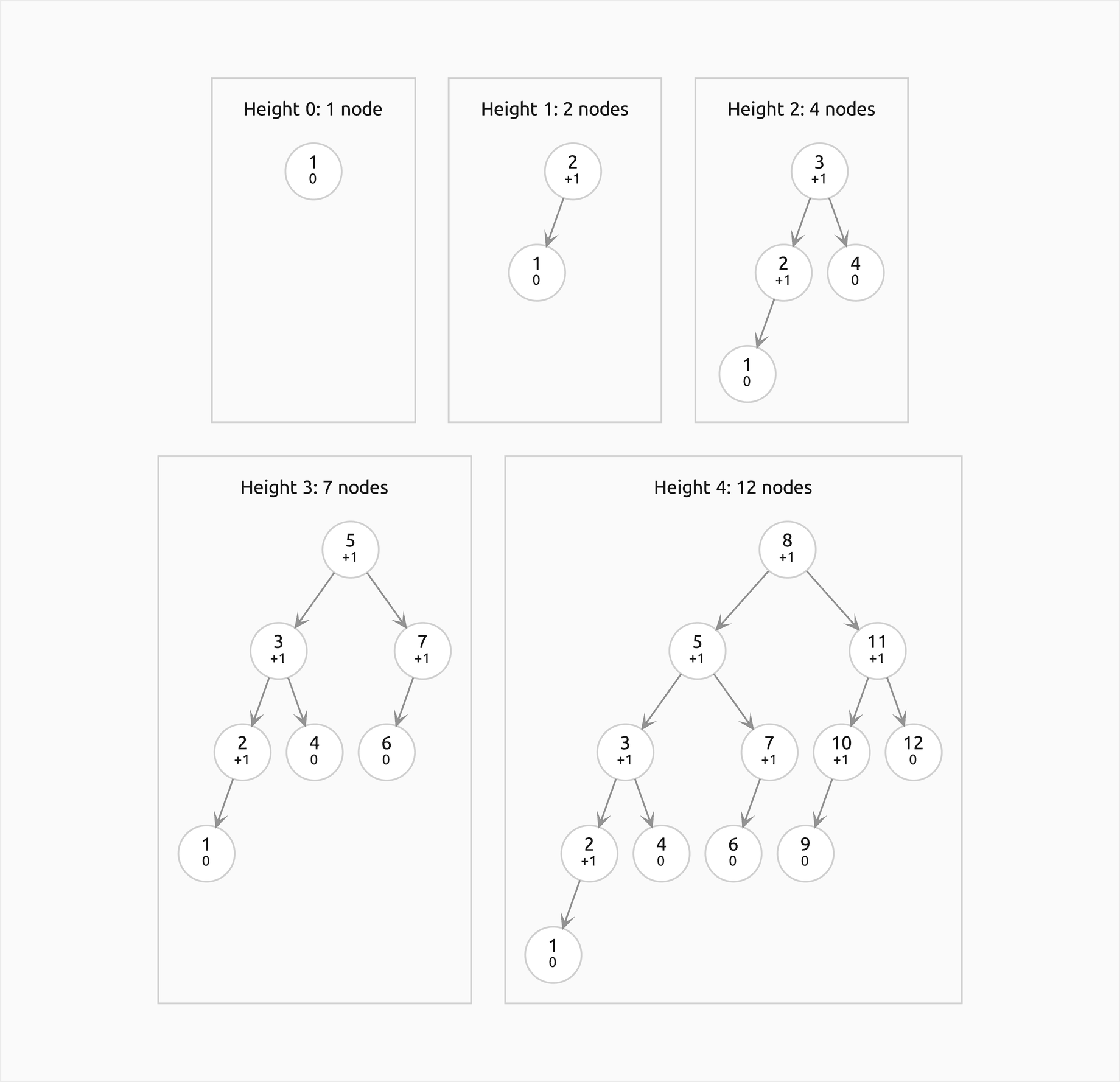
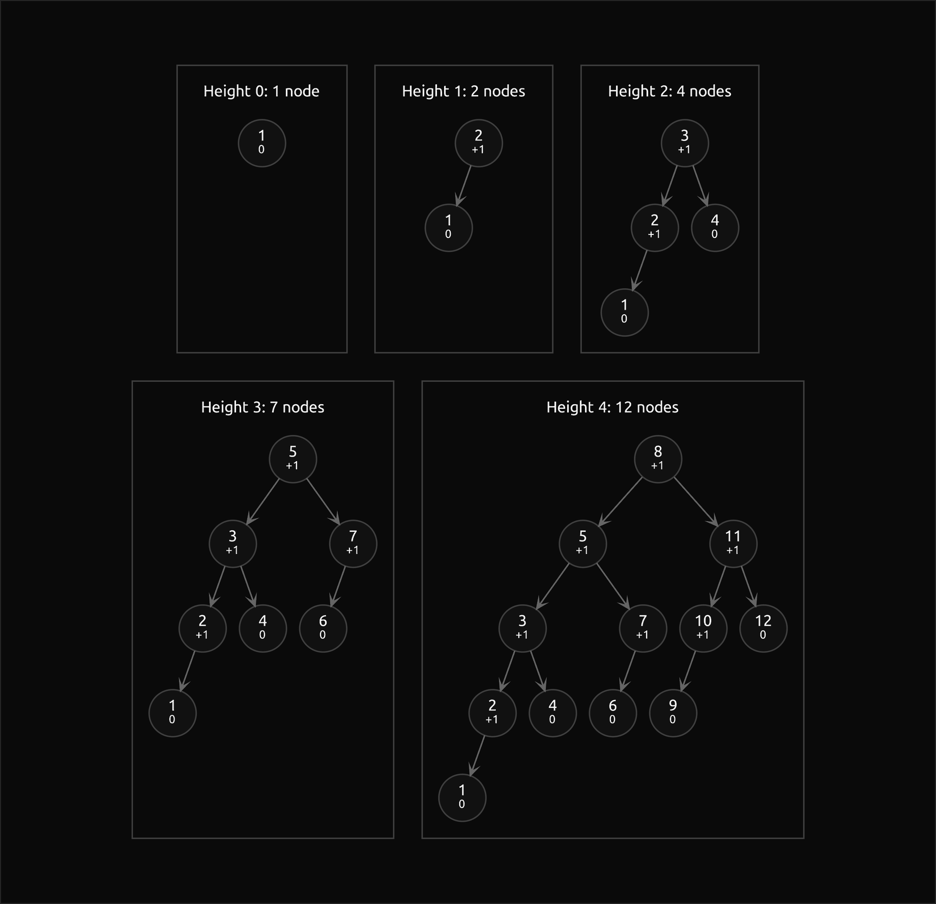
Every inner node of a sparsest tree is at +1, and the tree has no node to spare: with one node fewer, no AVL tree of that height exists. Binet's formula gives the Fibonacci numbers in closed form, and since the second term is less than 1 in size, it gives a lower bound:

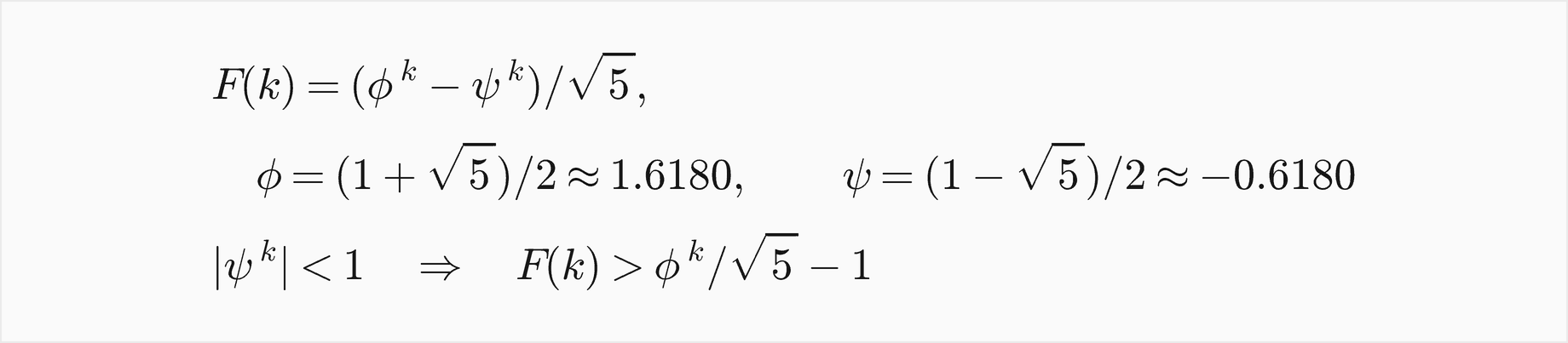
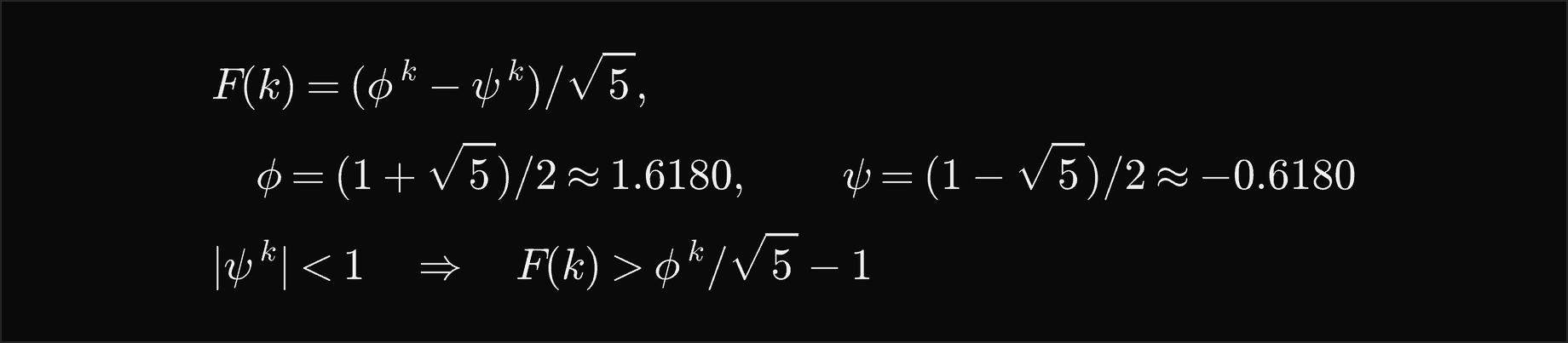
Now take any AVL tree of height h with n nodes. It has at least N(h) nodes, and solving for h gives the bound:

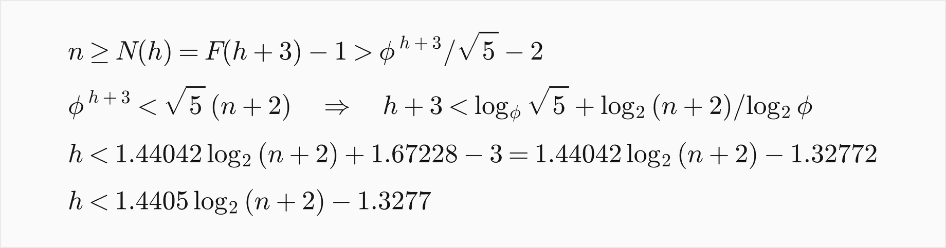
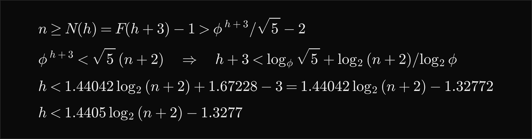
The factor 1/log2 φ is 1.44042..., and the classic statement rounds it up to 1.4405 and the constant up to −1.3277, which keeps the inequality true. Books that count height in nodes add one to both sides and quote the same bound as 1.4405 log2(n + 2) − 0.3277, with N(h) = F(h + 2) − 1. With the shortest possible height, that of a complete tree, the AVL height is pinned between two logarithms:

A complete tree is the shortest binary tree with n nodes, so no tree of any kind can be shorter than that.

So an AVL tree is never more than about 44 percent taller than the best possible tree. The example height_bound.py builds the sparsest tree of every height from 0 to 19 and counts its nodes, and computes the tallest possible height for each n exactly from N(h):

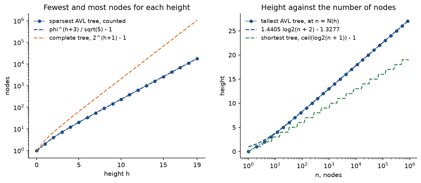
The bound is tight: at the sparsest trees, the tallest for their size, it exceeds the true height by as little as 0.0013 for heights up to 58. For a million keys an AVL tree has height between 19 and 27, and the bound gives 27.3837; for a billion, between 29 and 41.

Every operation

For an AVL tree of n keys and height h, with h < 1.4405 log2(n + 2) − 1.3277:

• search, contains, floor, ceiling, rank and select: at most h + 1 three-way comparisons, O(log n) in the worst case.
• min and max: O(log n), one path.
• range with k results: at most k + 2(h + 1) nodes visited, O(log n + k).
• insert: at most h + 1 comparisons, at most h + 1 nodes retraced, and at most one repair (one or two rotations), O(log n) in the worst case.
• delete: at most h + 1 comparisons plus the walk to the donor, at most h + 1 nodes retraced, and at most ⌊h/2⌋ repairs, O(log n) in the worst case.
• build from n keys: O(n log n) by insertions; from keys already sorted, a balanced tree can also be built directly in O(n).
• space: one node per key, with two pointers, a key, a value, a height and a size.

All of these bounds are worst case, for every single operation, which is what distinguishes balanced trees from structures such as splay trees, whose bounds are amortized, and from hash tables and treaps, whose bounds are expected.

Rotations per insertion and per deletion

The repair bound for deletion follows from heights along the path. Let v0 be the root, of height h, and vk the node physically removed, of height at least 0. A node on the path can need a repair only if the path enters its shorter subtree, which is two levels lower than the node; every other step of the path drops at least one level. With r repairs on a path of k steps:

The sparsest trees reach this bound: deleting the last node on their right side triggers a repair at every second level on the way up.

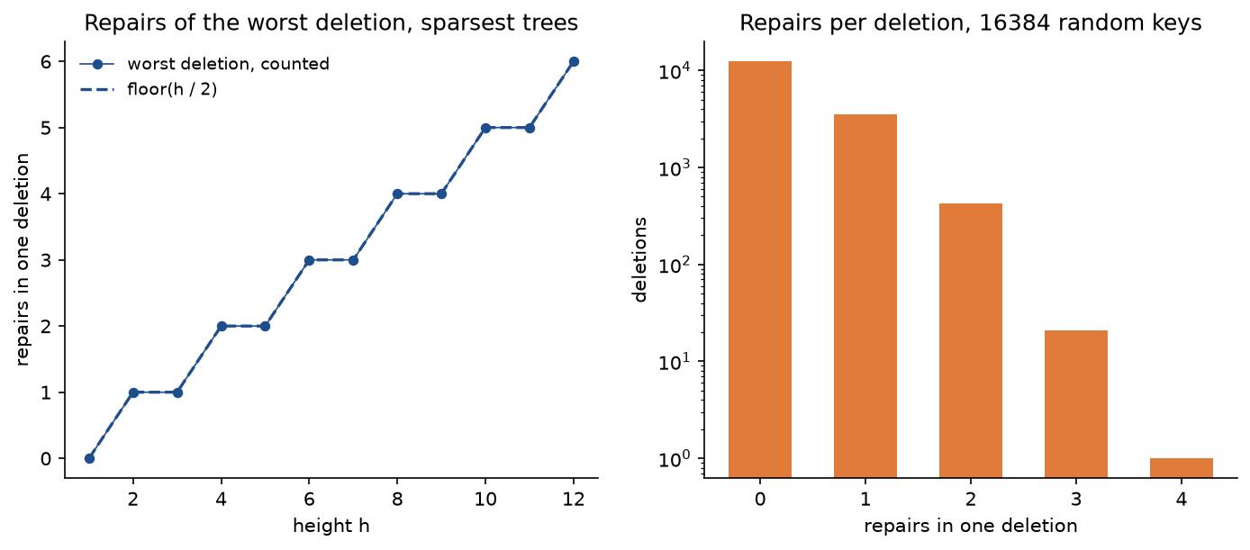
The worst case is rare. Draining a random AVL tree of 16384 keys in random order, 12429 deletions (0.7586) needed no repair, 3510 (0.2142) needed one, 423 (0.0258) needed two, 21 needed three and one deletion needed four; there were 0.3767 rotations per deletion on average.

Insertions never need more than one repair, and sorted input needs one almost every time. Inserting 1, 2, ..., n into an empty tree rotates once for every key except the powers of two: each power of two 2^k arrives when the 2^k − 1 keys before it form a perfect tree, and it only lengthens the rightmost path. So the count is exact:

For n = 16384 that is 16369 rotations, 0.9991 per insertion.

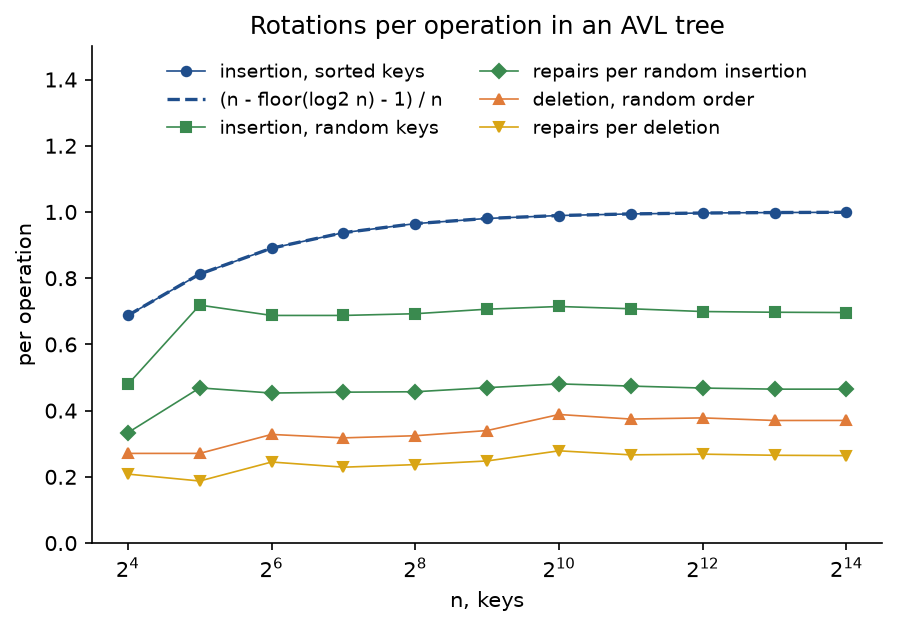
Random insertions make about 0.70 rotations, in 0.46 repairs, per insertion (0.6963 and 0.4649 at n = 16384, averaged over three seeds), and random deletions 0.3704 rotations in 0.2641 repairs. So the rebalancing work per update is a small constant on average; what costs O(log n) is the search and the retracing, and both are short.

Measured against a plain search tree

The example growth_against_bst.py inserts sorted keys and random permutations into both trees, records the height and the comparisons at every power of two up to 16384, and draws them over their predictions. For a plain tree, sorted keys cost 0 + 1 + ... + (n − 1) comparisons, and a random order costs the classical average:

That is (n − 1)/2 comparisons per insertion on average, 1023.5 at n = 2048, each one a step down the path.

Here H(n) is the n-th harmonic number, about ln n + 0.5772, so a randomly built plain tree costs about 39 percent more comparisons than log2 n, the cost in a perfectly balanced one.

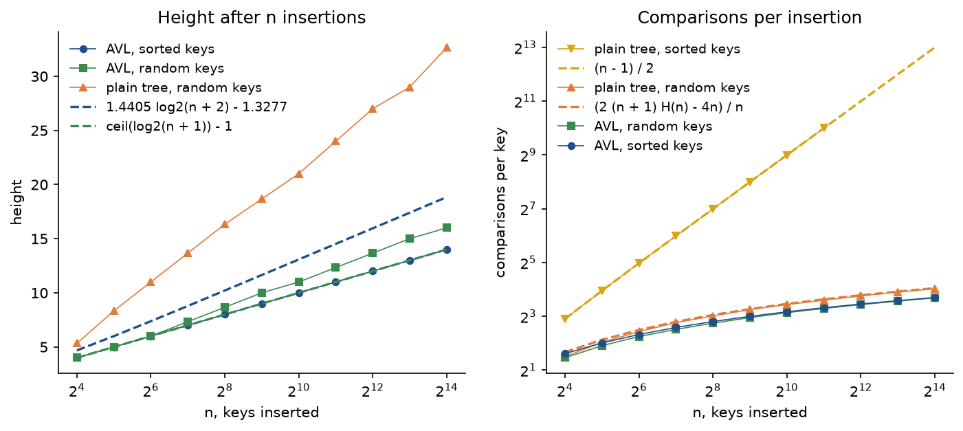
At n = 16384 the AVL tree built from sorted keys has height 14, the least possible, and from random keys 16 (the mean of three seeds), under the bound of 18.8396. The plain tree reaches 32.67 on random keys and 2047 on 2048 sorted or alternating keys. Per insertion, the AVL tree makes 13.0001 comparisons on sorted keys and 12.8737 on random ones, the plain tree 16.3284 on random keys and 1023.5 on 2048 sorted keys, with (n − 1)/2 = 8191.5 predicted at 16384. On random input the AVL tree saves only about a fifth of the comparisons; its value is that no input order can make it slow.

Worked example

Every step below is printed by examples/worked_example.py and asserted by tests/test_worked_example.py. Trees are written key(left subtree, right subtree), with a dash for an empty side and a leaf written as its key alone, so 39(34, 85(51, -)) is 39 with the leaf 34 on its left and, on its right, 85 with a left child 51. Balance factors are left height minus right height.

Inserting thirteen keys

The keys 85, 39, 34, 51, 56, 62, 96, 81, 21, 63, 99, 90 and 67 go into an empty AVL tree in that order.

• 85 becomes the root.
• 39 < 85, so 39 becomes the left child of 85. 85 is at +1: 85(39, -).
• 34 < 85, 34 < 39: left child of 39. Retracing, 39 is +1 and 85 is +2, unbalanced. y = 39 leans left, towards x = 34, so this is left-left: rotate right at 85, and 39 moves up: 39(34, 85). 39 is back at height 1, the height 85 had before.
• 51 > 39, 51 < 85: left child of 85. 85 is +1, 39 is −1: 39(34, 85(51, -)).
• 56 > 39, 56 < 85, 56 > 51: right child of 51. 51 is −1 and 85 is +2, but y = 51 leans right, towards x = 56: left-right. Rotate left at 51, giving 85(56(51, -), -), then right at 85: 39(34, 56(51, 85)). Two rotations, three comparisons.
• 62 > 39, 62 > 56, 62 < 85: left child of 85. 85 is +1, 56 is −1, and 39 is −2 with y = 56 leaning right: right-right. Rotate left at 39: 56(39(34, 51), 85(62, -)).
• 96 becomes the right child of 85, which becomes level, so retracing stops: 56(39(34, 51), 85(62, 96)).
• 81 > 56, 81 < 85, 81 > 62: right child of 62. 62 is −1, 85 is +1, 56 is −1.
• 21 goes left of 34. 34 and 39 are +1 and the root 56 becomes level.
• 63 > 56, 63 < 85, 63 > 62, 63 < 81: left child of 81. 81 is +1 and 62 is −2, with y = 81 leaning left, towards x = 63: right-left. Rotate right at 81, giving 62(-, 63(-, 81)), then left at 62, and 63 moves up: 56(39(34(21, -), 51), 85(63(62, 81), 96)). Four comparisons, two rotations.
• 99 becomes the right child of 96; 85 becomes level.
• 90 becomes the left child of 96, which becomes level.
• 67 > 56, 67 < 85, 67 > 63, 67 < 81: left child of 81, and every factor on the path stays within one.

The tree is now 56(39(34(21, -), 51), 85(63(62, 81(67, -)), 96(90, 99))), of height 4. The thirteen insertions took 33 comparisons and 6 rotations in 4 repairs, one of each case.

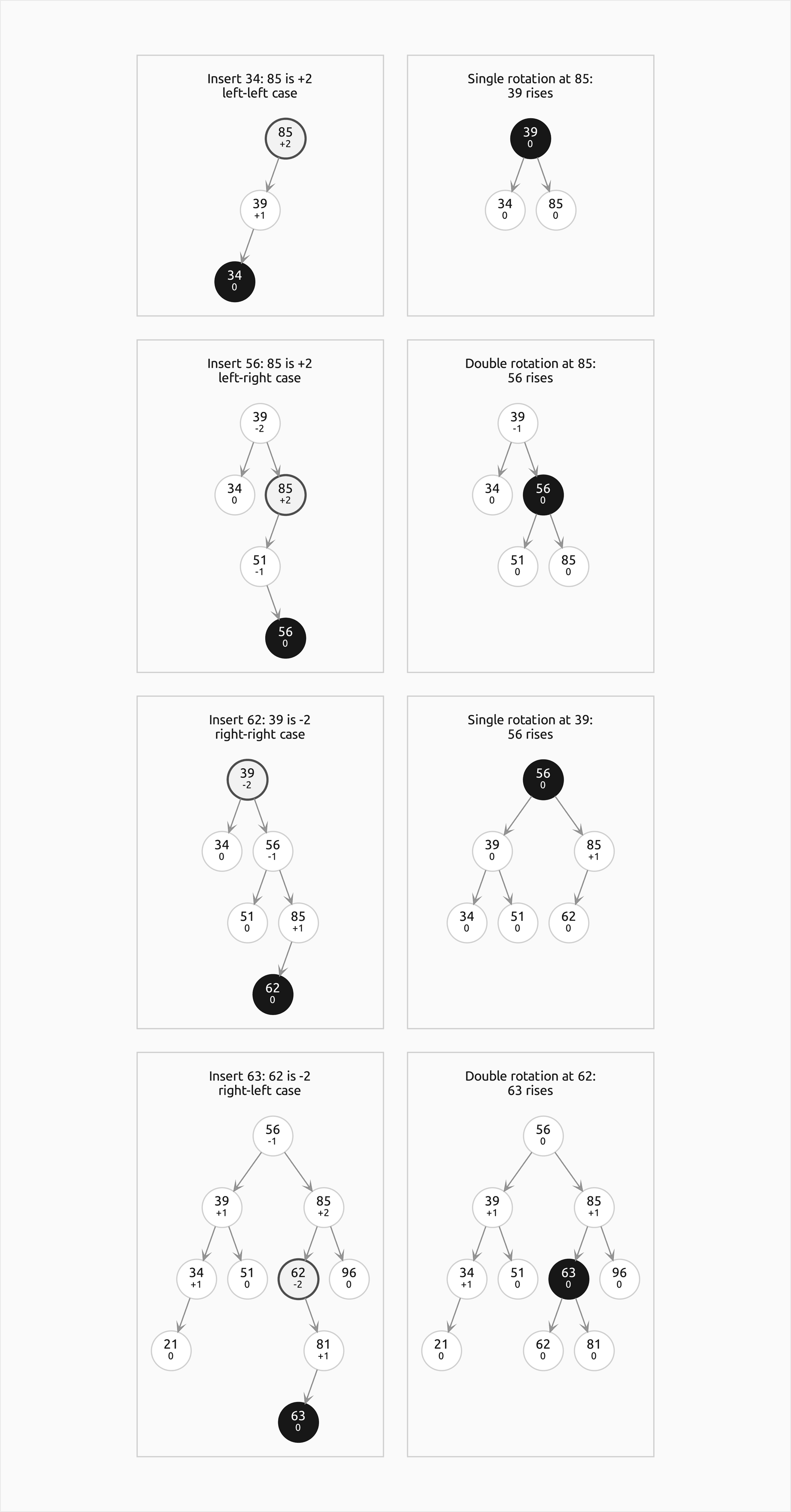
Each row shows, on the left, the tree with the unbalanced node outlined and the new key filled, then, on the right, the tree after the repair with the node that moved up filled. In every row the repaired subtree ends exactly as tall as it was before the insertion, which is why no node above it ever needed attention.

Deleting three keys

Then 90, 51 and 56 are deleted, with the successor rule for nodes with two children.

• Delete 90: four comparisons find the leaf 90, which is removed. 96 is now −1 but kept its height 1, so retracing stops at once. No repair.
• Delete 51: three comparisons find the leaf 51. Its parent 39 is left with 34(21, -) on its left and nothing on its right, so 39 is +2. y = 34 leans left: left-left, which the R and L naming calls R1. Rotate right at 39: 56(34(21, 39), 85(...)). The repaired subtree, now under 34, has height 1 where 39's had height 2, so retracing continues. The root 56 now has a left subtree of height 1 and a right subtree of height 3: −2. y = 85 leans left (+1), towards x = 63: right-left, or L1. Rotate right at 85, then left at 56, and 63 becomes the root: 63(56(34(21, 39), 62), 85(81(67, -), 96(-, 99))). One deletion, two repairs, three rotations, and the whole tree is one level lower.
• Delete 56: it has two children, so its successor 62, the leftmost node of its right subtree, takes its place, and the leaf 62 is removed from below. The node now holding 62 has 34(21, 39) on its left and nothing on its right: +2. y = 34 is level, the case only deletions produce, called R0. A single right rotation at 62 lifts 34: 63(34(21, 62(39, -)), 85(81(67, -), 96(-, 99))). The subtree under 34 has height 2, the height it had before, so retracing stops.

The final tree is 63(34(21, 62(39, -)), 85(81(67, -), 96(-, 99))), of height 3. With the predecessor rule, deleting 56 would have moved 39 up instead, and the final tree would be 63(39(34(21, -), 62), 85(81(67, -), 96(-, 99))): a different tree, equally valid. Hand-traced answers must say which rule they use.

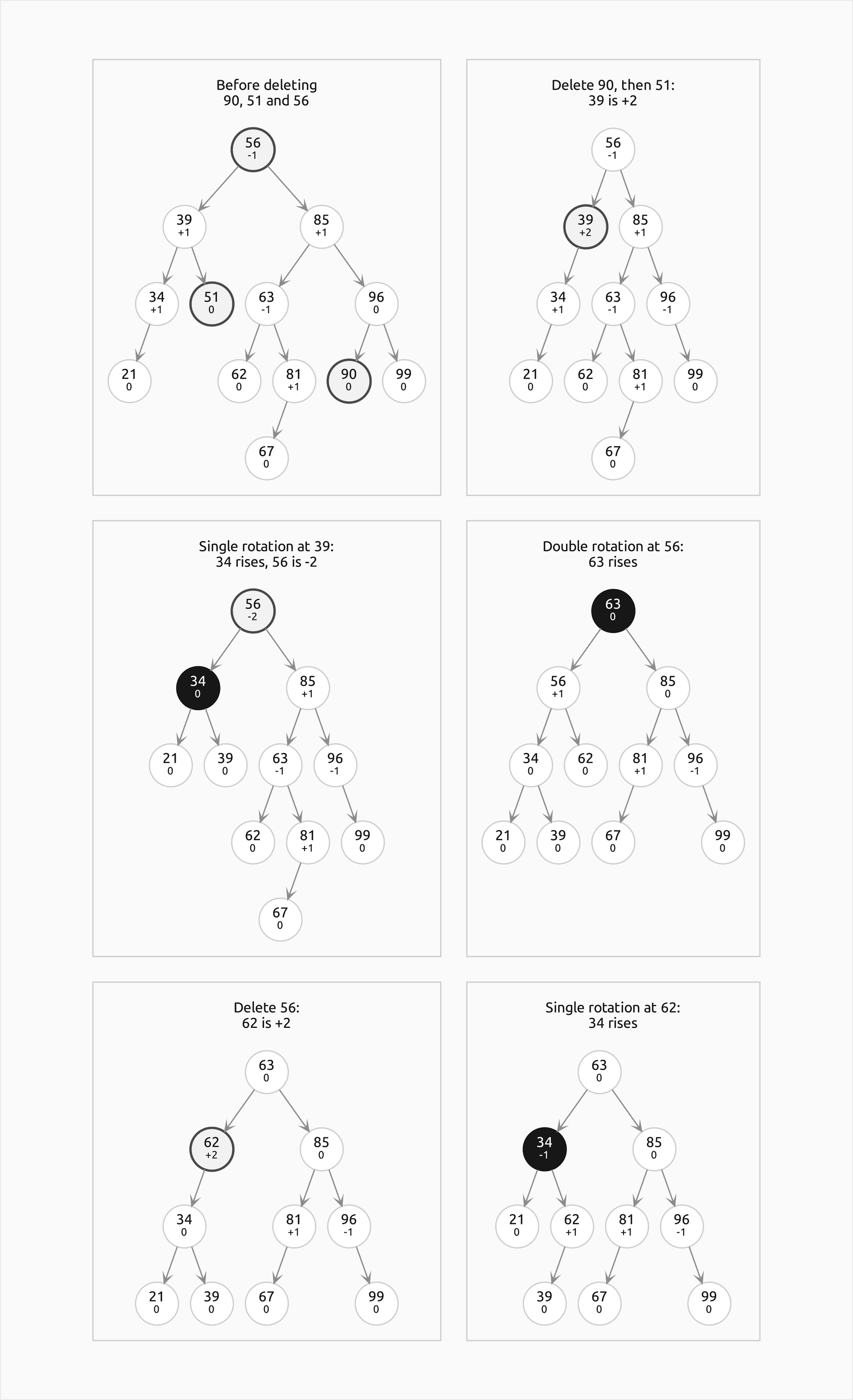
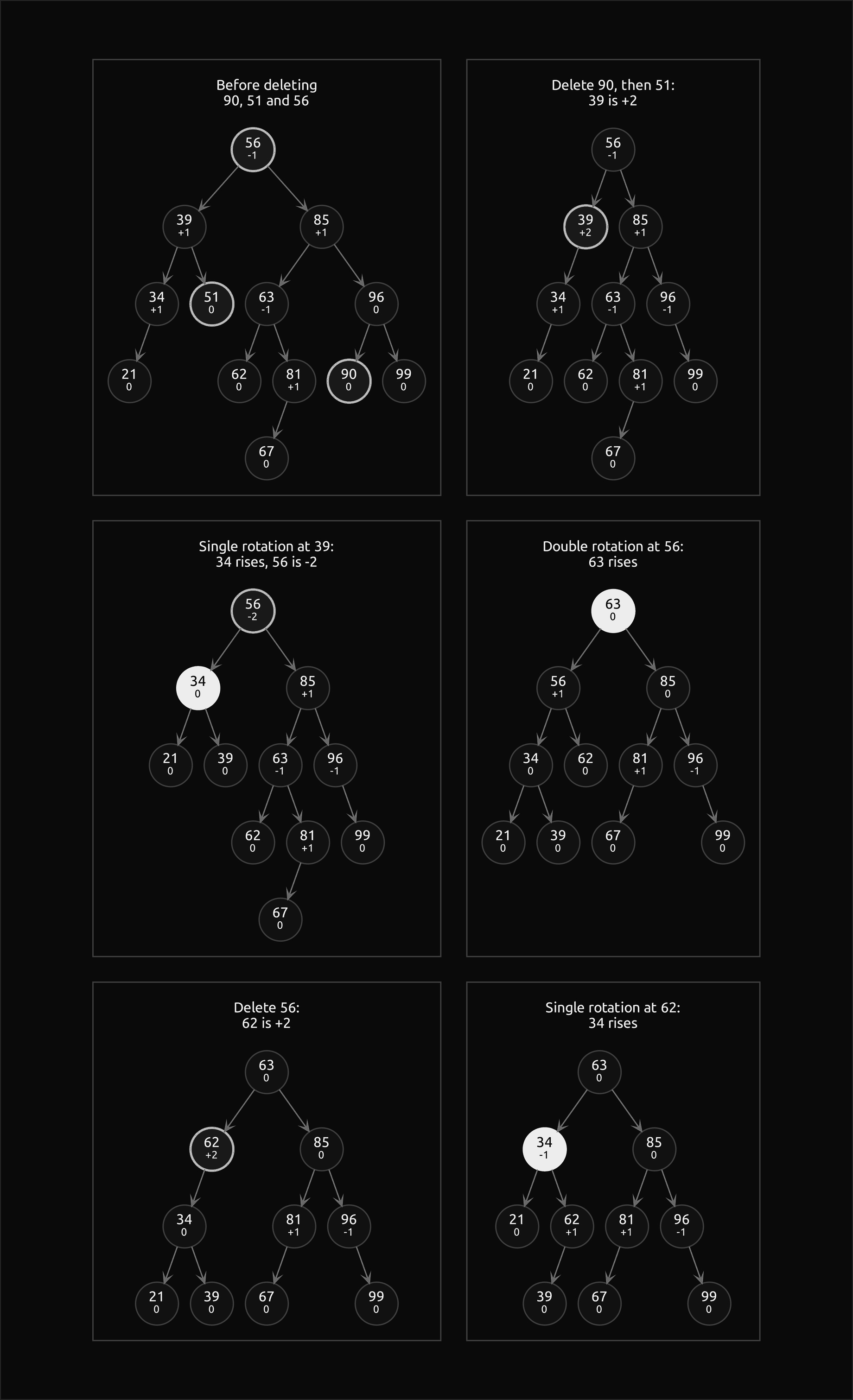
The second and third frames are the point of the example: the repair at 39 made its subtree shorter, which unbalanced the root, so one deletion needed repairs at two levels. The last row shows the level child, where the single rotation keeps the height and the walk stops.

The code

The package avl_trees is plain Python, one idea per module. Importing it needs only the standard library; Matplotlib is imported by plotting.py alone and sortedcontainers inside comparisons.py.

• node.py holds Node with its key, value, children, height and size, the convention (height counts edges, the factor is left minus right), balance_factor and update.
• counting.py holds OperationCounter, with the fields comparisons, rotations, rebalances (repairs), height_changes and visits, which every operation accepts or the tree carries, and CountedKey, which counts the less-than tests library code makes.
• trace.py holds the Step record, record, which appends a step to an optional trace list, describe and format_trace, which print the lines quoted above.
• shape.py converts trees to and from nested tuples and the key(left, right) text, measures any binary tree without recursion, and holds Subtree, a whole subtree drawn as a triangle, with the balance factors of a shape that contains them.
• rotations.py holds rotate_left and rotate_right; cases.py holds classify, taller_path, plan, rebalance and deletion_name.
• retrace.py holds retrace, the bottom-up walk shared by insertion and deletion, and restore_balance, the traced repair inside a whole tree.
• insertion.py and deletion.py hold descend, insert, delete and find_donor; tree.py holds AVLTree, the ordered map built on them, and queries.py its find, floor_node, ceiling_node, rank, select and range_nodes.
• bst.py holds BinarySearchTree, the plain iterative tree measured against; balance_factors.py holds BalanceFactorTree, the representation that stores factors.
• bounds.py holds the Fibonacci numbers, minimal_nodes, fibonacci_tree, max_height, min_height, the height bound and the repair and rotation counts derived above; growth.py holds the measurements behind the figures.
• invariants.py holds order_violation, avl_violation, is_avl, check_avl and the checks for factor-storing trees.
• workloads.py holds the worked example's keys and seeded random inputs: permutations, keys with repeats, sorted and alternating orders, and operation sequences that grow and drain the tree.
• layout.py places every node with a tidy tree layout that centres a parent over its children and keeps a left child on the left; drawing.py turns one state into Graphviz text with every node pinned at its place, balance factors under the keys and triangles for whole subtrees; frame_grid.py arranges states in rows, as one tree, a before and after pair or a grid; schematics.py builds the four case diagrams from real nodes and the package's own rotations.
• comparisons.py puts sortedcontainers next to the package; pitfalls.py holds deliberately broken versions for the pitfalls below; plotting.py draws every figure in the handbook's colours.

Counting and tracing never change what the code does. The whole of rebalancing is one loop over the path:

for index in range(len(path) - 1, -1, -1):
    node = path[index]
    if settled:
        update(node, counter)
        continue
    before = node.height
    update(node, counter)
    record(trace, "retrace", (node.key,), (node.height, balance_factor(node)))
    top = node
    if abs(balance_factor(node)) > 1:
        parent = path[index - 1] if index else None
        top = restore_balance(tree, parent, node, counter, trace)
    if top.height == before:
        settled = True

The examples run in a few seconds each from the repository root:

• examples/worked_example.py prints every step of the worked example and writes the six generated diagram sources: the four cases and the insertion and deletion traces.
• examples/height_bound.py builds the sparsest trees, checks the bound and finds the deletions with the most repairs.
• examples/growth_against_bst.py measures heights, comparisons and rotations against a plain search tree.
• examples/heights_or_balance_factors.py runs five seeded sequences of 4000 operations on both representations with both invariant checks after every operation, and compares their costs.
• examples/common_mistakes.py runs every broken version from pitfalls.py next to the correct code.
• examples/compare_with_sortedcontainers.py checks the package against SortedDict and counts the less-than tests of both.
• examples/practice.py prints fresh exercises with their solutions; --seed gives a new set.

python trees/avl-trees/examples/worked_example.py
python trees/avl-trees/examples/height_bound.py
python trees/avl-trees/examples/growth_against_bst.py
python trees/avl-trees/examples/heights_or_balance_factors.py
python trees/avl-trees/examples/common_mistakes.py
python trees/avl-trees/examples/compare_with_sortedcontainers.py
python trees/avl-trees/examples/practice.py --seed 7

The five sequences of heights_or_balance_factors.py pass through trees of up to 150 keys and back to empty, and both trees satisfy their invariants after every one of the 20000 operations, with identical shapes and identical rotations. Over 16384 random insertions both made 11259 rotations; the factor-storing tree adjusted 2.7786 factors per insertion and 1.8911 per deletion on its way back up, while the search path itself was 12.8046 nodes long. A Node with height and size takes 80 bytes in CPython and a BalanceNode 72, a difference that matters far less in Python than the two bits against six would in C.

The sample project, project/event_index.py with its helpers project/events.py and project/index.py, is an in-memory index of timestamped events, the kind a log collector or monitoring agent keeps for its most recent minutes. A seeded generator produces events in arrival order with bursts and random delays, so the stream is nearly sorted by time but not quite: in the default run of 120000 events, 51281 carry an earlier timestamp than the event before them. Each event is indexed by the key (timestamp, arrival number), which keeps equal timestamps distinct; a time t becomes the key (t, −1), which sorts before every event at t. Every 100 events, events older than the retention period (10 minutes by default) expire, each by deleting the minimum. Every 10 events a query asks for a time window (a range query), the number of events in it (two ranks), the last event before a time (a floor), the first one from a time (a ceiling), the number older than a time (a rank) and the n-th oldest live event (a select), and every answer is compared with an index on SortedDict. Options --events, --retention, --query-every, --bst-sample and --seed change the setup, and --figures writes the PNG elsewhere; the default run takes about 6 seconds.

python trees/avl-trees/project/event_index.py
python trees/avl-trees/project/event_index.py --events 300000 --retention 120000

In the default run 96326 events expire and 23674 remain. All 12000 queries agree with SortedDict, and the windows list 7241327 events between them. The index never grows taller than 15 for at most 25030 live events, under the bound of 19.7201 and one level above the least possible, and it makes 0.8624 rotations per insertion and 0.6737 per expiry.

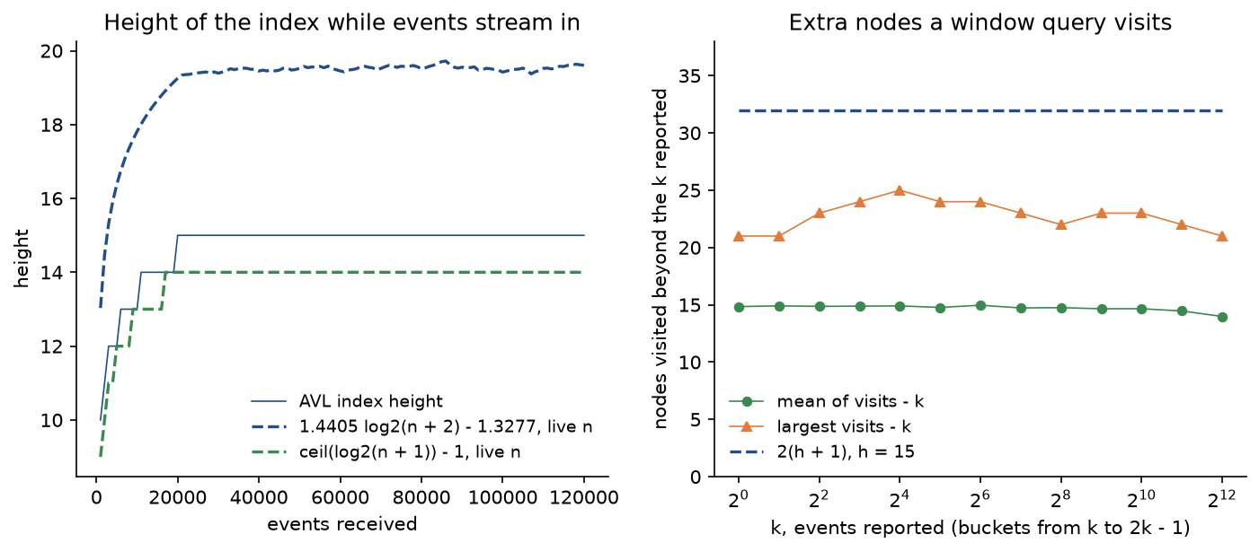
The right panel checks the range-query bound on real queries: whether a window holds 1 event or 4000, it costs the k reported nodes plus about 15 more, never more than 2(h + 1) = 32 more, and no window in the run exceeded k + 2(h + 1). The same events in a plain search tree show why the balancing matters here: the first 3000 events alone build a plain tree of height 1304 that needs 609.2 comparisons per insertion, because nearly sorted keys are almost the worst case for it.

The notebook avl_trees.ipynb follows this page: heights and factors, the four cases, insertion and deletion traced, the invariant under random operations, the height bound, the counted costs, the ordered queries next to sortedcontainers and a short run of the project. The tests in tests check the worked example tree by tree, the invariants after thousands of random operations, the bounds and exact counts claimed above, the agreement with sortedcontainers and with Python's sets and bisect, and every pitfall, and run in a few seconds:

python -m pytest trees/avl-trees

All data are synthetic, generated from seeds by workloads.py and project/events.py, so nothing is downloaded and no licence is involved.

In practice

sortedcontainers

Python has no balanced tree in its standard library. For a sorted list that rarely changes, bisect on a plain list gives O(log n) searches, but each insertion shifts on average half the list. The sortedcontainers package fills the gap with SortedList, SortedDict and SortedSet, which keep the items in a list of sorted sublists of up to a few thousand items each, plus an index of the sublists' maxima. A search is two binary searches; an insertion is a binary search and a short shift inside one sublist, which is a fast memory move in C. examples/compare_with_sortedcontainers.py shows that the two agree:

from avl_trees import AVLTree, floor_of, rank_of, sorted_dict

tree = AVLTree()
mapping = sorted_dict()
for key in (420, 150, 730, 310, 990, 505):
    tree[key] = mapping[key] = f"order {key}"
assert list(tree.items()) == list(mapping.items())
assert tree.floor(500) == floor_of(mapping, 500) == 420
assert tree.rank(500) == rank_of(mapping, 500) == 3
assert list(tree.irange(300, 600)) == list(mapping.irange(300, 600, inclusive=(True, False)))

On five random workloads of 6000 insertions, deletions and floor, ceiling, rank and membership queries, every answer and the whole contents after every operation agree. Counted through wrapped keys, SortedList needs fewer less-than tests: at n = 65536 it made 14.8127 per insertion and 16.0623 per search against the AVL tree's 22.1496 and 23.3486. A binary search asks one less-than question per step, while a search tree asks one or two at each node, depending on which way it turns; a tree can get down to one per level by testing only key < node.key on the way down and checking equality at the end. In wall-clock time the pure-Python AVL tree is about 12 times slower than SortedDict for 100000 insertions and searches, and the project's index about 9 times slower.

When to use which:

• Use a dict or set when you only need membership; it is O(1) expected and far faster than any ordered structure.
• Use bisect on a list for sorted data that is built once and then only searched.
• Use sortedcontainers in Python for an ordered map or set with frequent updates, floor and ceiling, ranks and ranges.
• Write a balanced tree when you need what a library container does not give: a worst-case bound on every single operation, augmentation (interval trees, order statistics over arbitrary values, sums over ranges), persistence by path copying, or the structure inside a language or system without such a library.

AVL or red-black

The red-black tree is the other classical balanced binary search tree, and the one most standard libraries chose. Its rule is looser, which bounds its height by 2 log2(n + 1) instead of 1.44 log2(n + 2), so searches in an AVL tree pass slightly fewer nodes in the worst case. In exchange a red-black tree does less restructuring: at most two rotations per insertion and three per deletion, against at most two for an AVL insertion and up to about h/2 repairs for an AVL deletion, although on average both trees rotate rarely, as the measurements above show. Both do O(log n) work per update in the worst case, both store one extra small field per node, and neither is simpler to implement in any meaningful way; the case analysis of red-black deletion is usually considered the harder of the two. A common rule of thumb follows from these numbers: AVL trees suit lookup-heavy workloads, red-black trees update-heavy ones, and for most programs the difference is small next to memory layout, which is why databases and file systems use B-trees instead of either. Later variants blend the two: the weak AVL (WAVL) tree of Haeupler, Sen and Tarjan behaves as an AVL tree while there are only insertions and never does more than two rotations per deletion.

Elsewhere

C++'s std::map and std::set in the major standard libraries and Java's TreeMap and TreeSet are red-black trees, as is the Linux kernel's rbtree, which its scheduler, timers and many other subsystems use. AVL trees appear where lookups dominate or where a generic in-memory ordered structure is needed: OpenZFS (from illumos) has a generic AVL tree library used throughout the file system, the Windows kernel offers AVL-based generic tables to drivers, and LLVM's immutable sets and maps are persistent AVL trees that share unchanged subtrees between versions. OCaml's standard Set and Map are height-balanced trees in the AVL family that allow a height difference of two. Rust's BTreeMap is a B-tree, chosen for cache behaviour, and Haskell's Data.Map uses weight-balanced trees, which balance subtree sizes instead of heights. Randomized alternatives, treaps and skip lists, give the same O(log n) bounds in expectation with simpler code, and splay trees give them amortized while adapting to the access pattern.

Pitfalls

• Mixing balance factor conventions. With left minus right a left-leaning node is +1; with right minus left it is −1. Rule tables for the deletion cases (R0, R1, R−1 and L0, L1, L−1) are written for one sign, and read with the other they swap the single and double rotations: in examples/common_mistakes.py, deleting 77 from 77(44(-, 49), 78) leaves 78(44(-, 49), -), a left-right case, and the mixed reading makes a single rotation that leaves 44(-, 78(49, -)), still unbalanced at −2. Write your convention down; the sign-free rule is "same lean or level: single; opposite lean: double".
• Using a single rotation for an inside case. Inserting 81, 26 and 63 makes 81 left-right, and a single right rotation only moves the problem to the other side: 26(-, 81(63, -)), now at −2. Inside cases need two rotations.
• Repairing the wrong node. Retracing must repair the lowest unbalanced node on the path, the first one found going up. Repairing the highest one instead leaves the lower one unbalanced, as the insertion of 44, 52, 86, 71, 59, 69, 89 and 93 shows, where 86 is left at −2.
• Updating heights in the wrong order. After a rotation the node that went down must be updated before the node that came up, whose height is computed from it. The other order stores a stale height at once: after inserting 85, 39 and 34 the tree looks right, 39(34, 85), but 39 stores height 3 where its subtrees give 1, and later repairs decide on wrong numbers.
• Stopping deletion after the first repair, as insertion may. In the worked example, deleting 51 needs a repair at 39 and then another at the root; stopping after the first leaves the root at −2.
• Retracing from the wrong node after a two-child deletion. The walk starts at the donor's old parent, not at the node whose key was named; starting higher leaves stale heights in between, as deleting 48 from 48(24, 72(57, -)) shows, where 72 keeps height 1 after losing its child.
• Using a double rotation when the child is level. After a deletion the taller child y can be level, and then only a single rotation is right. Deleting 56 from the tree built from 95, 88, 71, 56, 87, 21, 84 and 89 with a double rotation leaves 88 at −2.
• Forgetting which donor you use. The successor and predecessor rules give different trees, both valid; the worked example ends differently with each. When tracing by hand, state the rule, and remember that the repair cases are decided at the donor's old position.
• Reading a tree's balance only at the root. A tree whose root is level can still be badly unbalanced lower down; the AVL condition is about every node, and so is any check of it.
• Checking the order only between parents and children. 52(31(-, 67), 74) passes that check, but 67 sits in the left subtree of 52 while being larger; a correct check carries bounds from the ancestors down.
• Recursing along the paths of a plain search tree. Recursive insertion into a plain tree with sorted keys hits Python's recursion limit after about a thousand keys; an AVL tree's height stays small enough for recursion, but a plain tree used for comparison needs loops.
• Quoting the bound for the other height convention. With heights counted in nodes (a leaf 1, the empty tree 0) the bound reads h < 1.4405 log2(n + 2) − 0.3277, the form many books quote. Applied to edge-counted heights it allows one level too many; the edge-counted form applied to node-counted heights is simply false: the sparsest AVL tree with 33 nodes has 7 levels, height 6 in edges, while 1.4405 log2(35) − 1.3277 is 6.06. State which height you mean, and carry the shift through N(h) = F(h + 3) − 1 against F(h + 2) − 1 as well.

Further reading

• G. M. Adelson-Velsky and E. M. Landis, "An algorithm for the organization of information", Doklady Akademii Nauk SSSR 146(2), 263-266, 1962; English translation in Soviet Mathematics Doklady 3, 1259-1263, 1962. The original AVL tree.
• D. E. Knuth, The Art of Computer Programming, volume 3, Sorting and Searching, second edition, section 6.2.3, Addison-Wesley, 1998. Balanced trees, the height bound through Fibonacci trees, and the average number of rotations.
• T. H. Cormen, C. E. Leiserson, R. L. Rivest and C. Stein, Introduction to Algorithms, third edition, chapter 13 and problem 13-3, MIT Press, 2009. Red-black trees, and AVL trees as an exercise.
• R. Sedgewick and K. Wayne, Algorithms, fourth edition, section 3.3, Addison-Wesley, 2011. Balanced search trees through 2-3 trees and left-leaning red-black trees.
• L. J. Guibas and R. Sedgewick, "A dichromatic framework for balanced trees", Proceedings of the 19th Symposium on Foundations of Computer Science, 8-21, 1978. Red-black trees, and AVL trees seen in the same framework.
• K. Mehlhorn and A. Tsakalidis, "An amortized analysis of insertions into AVL-trees", SIAM Journal on Computing 15(1), 22-33, 1986. Why the balance changes per insertion are constant on average.
• B. Haeupler, S. Sen and R. E. Tarjan, "Rank-balanced trees", ACM Transactions on Algorithms 11(4), article 30, 2015. Weak AVL trees and a unified view of AVL and red-black trees.
• L. Devroye, "A note on the height of binary search trees", Journal of the ACM 33(3), 489-498, 1986. The expected height of a randomly built plain search tree.
• B. Pfaff, "Performance analysis of BSTs in system software", Proceedings of ACM SIGMETRICS, 2004. AVL, red-black and splay trees measured on real workloads.
• G. Jenks, the sortedcontainers documentation, especially its notes on implementation and performance at scale.