Single-source shortest paths¶

A navigation app looking for the quickest way home, a router deciding where to forward a packet, a trader looking for a chain of currency exchanges that ends with more money than it started with, and a project planner asking for the earliest possible finish are all asking one question: in a graph whose edges carry weights, which path from one vertex to each other vertex has the smallest total weight? This page defines that problem and the single operation every algorithm for it is built from, relaxation, and proves the properties that make relaxation work. It then derives Dijkstra's algorithm with a binary min-heap and proves it correct, shows the one negative edge that breaks it, replaces it by Bellman-Ford when weights can be negative, detects and extracts negative cycles, solves directed acyclic graphs in linear time, and extends Dijkstra to A for a single target with a heuristic. Afterwards you will be able to fill in the table of tentative distances and parents by hand for each algorithm, implement and test them, read paths back from parent pointers, and choose between Dijkstra, Bellman-Ford, the DAG algorithm, breadth-first search, A and the routines of NetworkX and SciPy. It builds on Graphs and their representations, Breadth-first and depth-first search and the indexed heap of Heaps and priority queues.

The algorithms need only the standard library and the indexed heap of the heaps topic; to run the plots and the notebook install the base group, and the graphs group for the comparisons with NetworkX and SciPy.

Intuition¶

Build a model of an undirected graph out of string: a knot for every vertex and, for every edge, a piece of string as long as its weight. Hold the knot of the source and lift the model slowly off the table. The knots leave the table one at a time, nearest first, and when the whole model hangs free every knot sits at a depth equal to its distance from the source. The strings pulled taut are the shortest paths; a slack string is an edge that no shortest path uses. Dijkstra's algorithm lifts the knots off the table in exactly this order.

A second picture fits every algorithm on this page. Each vertex keeps the length of the best route to it found so far, starting at infinity, and the algorithm keeps asking one question about an edge u→v: is going through u better than the best route to v known so far? If it is, v's number goes down and u becomes v's parent. That question is called relaxing the edge, and the algorithms below differ only in which edges they ask about, and in what order.

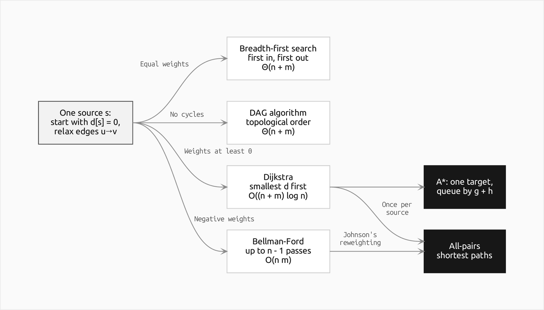
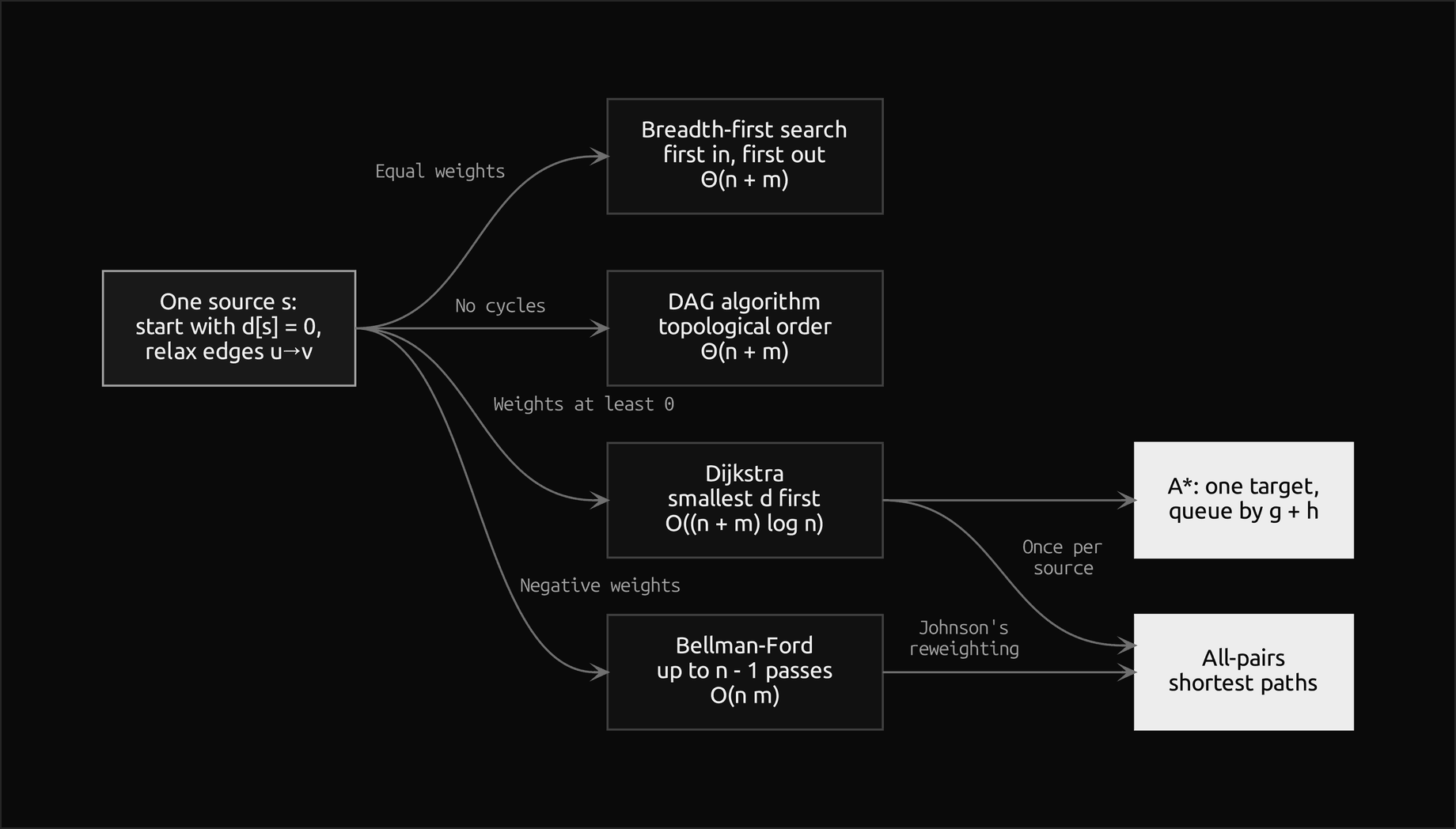
The map shows which algorithm fits which graph. Breadth-first search, the DAG algorithm and Dijkstra relax every edge exactly once, in an order that guarantees each relaxation uses a final distance; Bellman-Ford gives up on finding such an order and relaxes every edge again and again until nothing changes, which is slower but survives negative weights.

How it works¶

The problem¶

A weighted directed graph has n vertices, m edges and a weight w(u, v) on every edge u→v. The weight of a path is the sum of its edge weights:

The weight of a path p from v0 through v1 to vk is the sum, for i from 1 to k, of the weight of the edge from v i minus 1 to v i

The distance from a source s to a vertex v is the smallest weight of any path from s to v, and infinity when there is none:

delta of s and v is the minimum weight over all paths from s to v, and infinity when no path leads from s to v

The single-source problem asks for δ(s, v) for every vertex v, together with a shortest path to each. Three relatives reduce to it or build on it. The single-target problem is the single-source problem on the graph with every edge reversed. The single-pair problem, from s to one t, has no algorithm that is faster in the worst case than solving for every vertex, but it can stop early and, with A*, look mostly in the right direction. The all-pairs problem has its own page, All-pairs shortest paths. An undirected graph is a directed graph with each edge present in both directions.

Weights may be negative. A graph may then contain a negative cycle, a cycle of negative total weight; going round it once more always gives a lighter walk, so the vertices reachable from it have no shortest path at all, and their distance is −∞. Every algorithm here either refuses negative weights (Dijkstra and A*), cannot meet a cycle at all (the DAG algorithm), or detects negative cycles (Bellman-Ford).

The package represents a graph by a small class, WeightedDigraph, which keeps the vertices in insertion order and, for each vertex, a list of its out-edges as (head, weight) pairs, plus one list of all edges in insertion order. Vertices can be any hashable values, parallel edges are allowed, and weight(u, v) returns the lightest edge from u to v, the only one a shortest path would ever use. The order of the input decides the order of every trace, which is what makes the hand traces below reproducible.

Optimal substructure¶

Every part of a shortest path is itself a shortest path. If some subpath from x to y could be replaced by a lighter one, the replacement would make the whole path lighter, which contradicts its being shortest. Applied to the last edge of a shortest path, this says that a shortest path to v is a shortest path to its second-to-last vertex u followed by the edge u→v:

If p, from s through u to v, is a shortest path, then its prefix from s to u is a shortest path to u, and delta of s and v equals delta of s and u plus the weight of u to v

and that no edge offers a shortcut, the triangle inequality:

delta of s and v is at most delta of s and u plus the weight of u to v, for every edge u to v

Optimal substructure is why one parent per vertex is enough to store a shortest path to every vertex. If each reachable vertex remembers the vertex before it on one shortest path, the parents form a tree rooted at s, the shortest-path tree, and the path to any vertex is read by walking up the tree. n parents describe n paths whose total length can be quadratic in n. The argument needs one condition: no negative cycle reachable from s, because otherwise the shortest path does not exist.

Relaxation and its properties¶

Every algorithm keeps a tentative distance d[v] and a parent for every vertex. Initially d[s] = 0, every other d[v] is ∞ and no vertex has a parent. Relaxing the edge u→v is the test and update:

If d of u plus the weight of u to v is less than d of v, then d of v becomes d of u plus that weight, and the parent of v becomes u

The test is strict: an equally good route never replaces the parent already recorded. Relaxation is the only place where a distance changes, so a handful of properties hold for every algorithm on this page, whatever order it relaxes edges in:

Upper bound. d[v] is always the weight of some walk from s to v, or ∞, so it is never below δ(s, v); and once it equals δ(s, v), no relaxation can lower it further.
No path. If v cannot be reached from s, d[v] stays ∞ for ever.
Convergence. If u→v is the last edge of a shortest path to v and d[u] is already correct when u→v is relaxed, then d[v] is correct afterwards, by the substructure equation above.
Path relaxation. If the edges of a shortest path are relaxed in path order, with any other relaxations mixed in, the last vertex ends with its correct distance. This follows from convergence, edge by edge along the path.
Parent tree. Once every d[v] is correct, the parent pointers form a shortest-path tree.

The upper bound holds because a relaxation only ever replaces d[v] by the weight of an actual walk, d[u] plus one more edge:

d of v is at least delta of s and v for every vertex at every moment, and once d of v equals delta of s and v no relaxation changes it again

Convergence turns one correct distance into the next one along a shortest path:

If the path from s through u to v is shortest and d of u equals delta of s and u before u to v is relaxed, then d of v equals delta of s and v after it

and path relaxation chains it along the whole path, which is all an algorithm has to arrange:

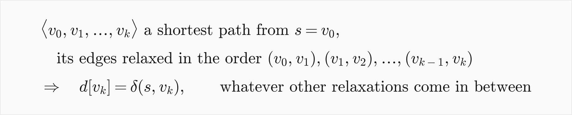
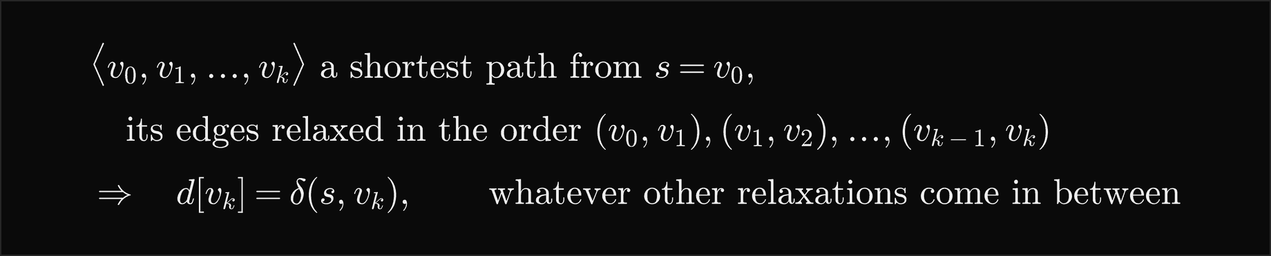
If v0 to vk is a shortest path from s equal to v0 and its edges are relaxed in the order v0 v1, v1 v2, up to v k minus 1 v k, then d of v k equals delta of s and v k, whatever other relaxations come in between

The three properties are the whole correctness argument of the DAG algorithm and of Bellman-Ford, and the key step of Dijkstra's. They also give a certificate that is far easier to check than the answer was to find. If d[s] = 0, no edge is tense (no relaxation would change anything) and every reached vertex's parent edge is tight (d[v] equals d[parent] plus the edge's weight) on a parent chain leading back to s, then every d[v] is at most the weight of every path to v and equal to the weight of one, so it is the distance. shortest_paths_violation in invariants.py checks exactly this and names the first broken condition; the tests run it on the answers for about a hundred random graphs, with and without negative weights.

Dijkstra's algorithm¶

When no weight is negative, there is an order in which every edge needs to be relaxed only once: settle the vertices in increasing order of distance. Dijkstra's algorithm keeps the vertices that have been reached but not settled in a min-priority queue keyed by their tentative distance, and repeats:

Extract the vertex u with the smallest key. It is now settled: its distance is final.
Relax every edge u→v. If v's distance drops and v is waiting in the queue, decrease its key; if v was never reached, push it.

The queue must be a min-priority queue. A max-priority queue would hand out the vertex with the largest tentative distance, the one least likely to be final, and the results are simply wrong: on the worked example below it returns 14 instead of 4 for A. The package uses the IndexedHeap of the heaps topic, a binary min-heap with a map from each item to its array position, so that decrease-key finds the vertex in O(1) and sifts it up in O(log n). Stripped of its counting and tracing, the main loop is:

while queue:
    vertex, key = queue.pop()
    settled.add(vertex)
    if vertex == target:
        break
    for head, weight in graph.out_edges(vertex):
        if not relax(vertex, head, weight, distance, parent, counter, trace):
            continue
        if head in queue:
            queue.decrease_key(head, distance[head])
        elif head not in settled:
            queue.push(head, distance[head])

The invariant is that every extracted vertex has its final distance. Suppose not, and let u be the first vertex extracted with d[u] > δ(s, u). Some shortest path leads from s to u; let y be the first vertex on it that was not yet extracted when u was, and x the vertex just before y, which was extracted earlier with its correct distance. When x was extracted its edge x→y was relaxed, so by convergence d[y] = δ(s, y). Then:

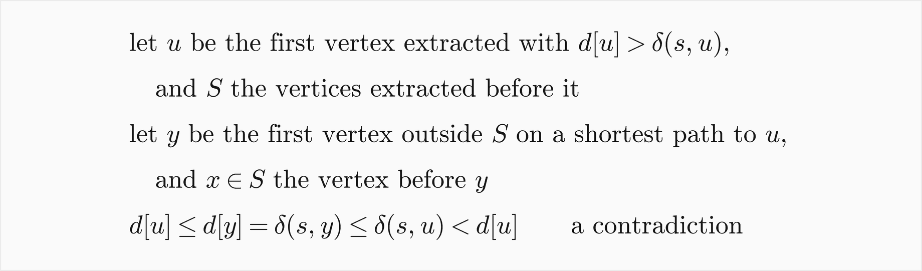
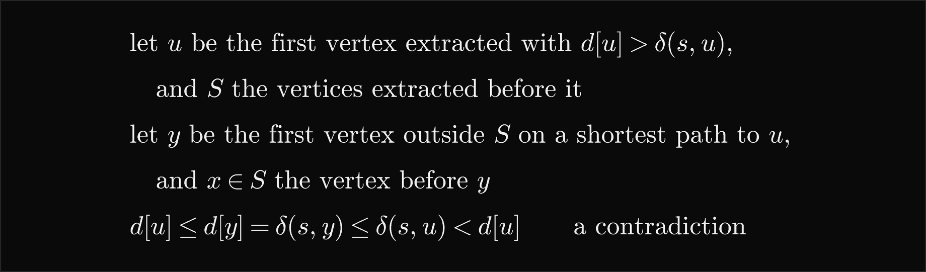
Let u be the first vertex extracted with d of u greater than delta of s and u, and S the vertices extracted before it; let y be the first vertex outside S on a shortest path to u, and x in S the vertex before y; then d of u is at most d of y, which equals delta of s and y, which is at most delta of s and u, which is less than d of u, a contradiction Let u be the first vertex extracted with d of u greater than delta of s and u, and S the vertices extracted before it; let y be the first vertex outside S on a shortest path to u, and x in S the vertex before y; then d of u is at most d of y, which equals delta of s and y, which is at most delta of s and u, which is less than d of u, a contradiction

The first inequality holds because u was extracted while y was still in the queue, so u's key was the smaller; the equality is convergence; the second inequality holds because y lies on a shortest path to u and the rest of that path has weight at least zero. That last step is the only place the proof uses the absence of negative weights, and it is exactly where a negative edge breaks the algorithm. Because extracted distances are final, the keys come out of the queue in nondecreasing order, every vertex is extracted once, and every edge is relaxed once. With a target, the run can stop as soon as the target is extracted.

The algorithm is greedy: it commits to the nearest unsettled vertex and never revisits the choice, and the proof above is its exchange argument (see Greedy algorithms). Prim's algorithm in Minimum spanning trees has the same shape with the key d[u] + w(u, v) replaced by w(u, v).

Why a negative edge breaks it¶

Four vertices are enough. With the edges S→A of weight 2, S→B of 5, A→C of 4 and B→A of −4, Dijkstra extracts S, then A with distance 2 and sets C to 2 + 4 = 6, then B with distance 5. Relaxing B→A now offers 5 − 4 = 1 < 2, but A is settled: its out-edge was relaxed with the old distance and is never relaxed again. C is extracted with 6, although S→B→A→C weighs 5.

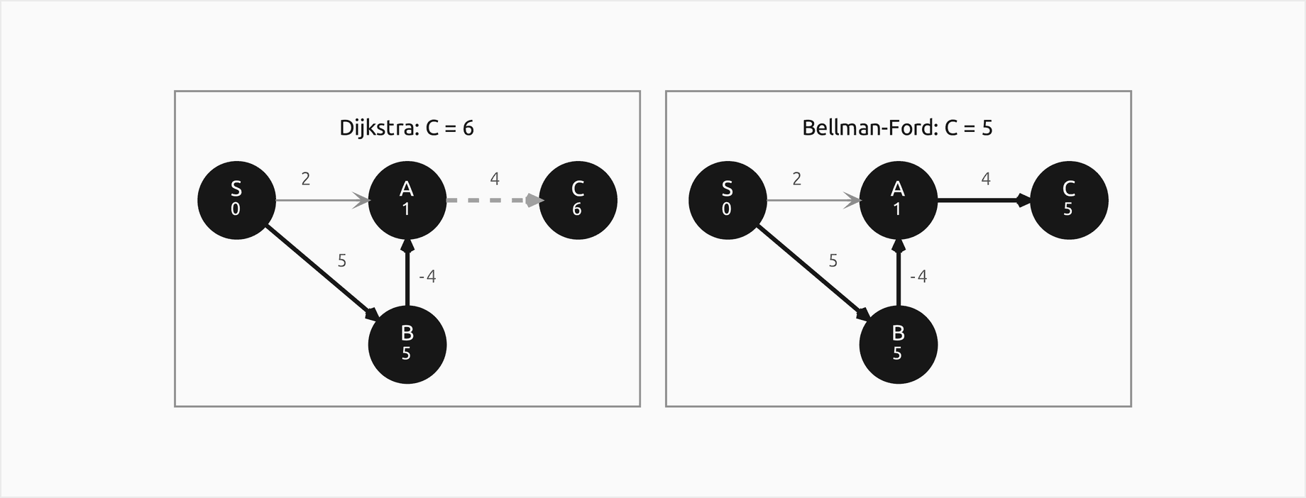
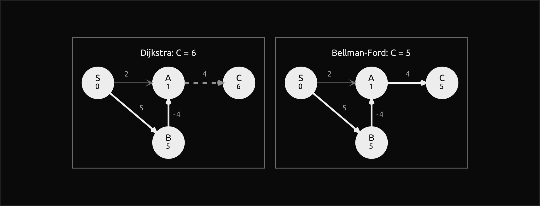
Two frames of the four-vertex graph, S, A and C along the top and B below A, every vertex filled because both algorithms have finished with it and the parent edges bold: on the left, Dijkstra's answer with A at 1 via B but C still at 6, and the edge A to C dashed and bold because it is still tense; on the right, the true distances found by Bellman-Ford, with C at 5 via A Two frames of the four-vertex graph, S, A and C along the top and B below A, every vertex filled because both algorithms have finished with it and the parent edges bold: on the left, Dijkstra's answer with A at 1 via B but C still at 6, and the edge A to C dashed and bold because it is still tense; on the right, the true distances found by Bellman-Ford, with C at 5 via A

The left frame is what the package's dijkstra(..., allow_negative=True) returns: the certificate check finds the edge A→C still tense, d[C] = 6 > d[A] + 4. The proof fails at the step δ(s, y) ≤ δ(s, u): the path to A through B is longer in edges but lighter, because its last edge is negative. Two tempting repairs do not work. Adding 4 to every weight makes them all nonnegative, but a path pays the 4 once per edge, so paths with more edges are punished; on this graph the shortest path to A becomes S→A instead of S→B→A. And letting a settled vertex back into the queue gives correct answers whenever there is no negative cycle, but it can take exponential time, and on a negative cycle it never ends. Bellman-Ford is the honest answer. By default the package refuses negative weights with a NegativeWeightError; NetworkX raises a ValueError when it notices the contradiction a negative edge causes.

Two other queues: lazy deletion and a plain list¶

Python's heapq has no decrease-key. dijkstra_lazy therefore pushes a new entry (distance, sequence number, vertex) every time a distance drops and leaves the old entry in the heap. When an entry comes off the heap with a key larger than its vertex's current distance, it is stale, and it is skipped. Every push follows a strict improvement, so exactly one entry per vertex is live. The heap can hold up to m + 1 entries instead of n, which costs memory and makes every heap operation work on a larger heap, but the code is short and the constant factors of heapq are small; on the worked example it makes 9 pushes and skips 3 stale entries.

dijkstra_array drops the heap altogether: the unsettled vertices sit in a plain list and each extraction scans all of them for the smallest distance. That is Θ(n) per extraction and Θ(n²) in all, which sounds worse than a heap until the graph is dense: with m close to n², relaxing the edges costs Θ(n²) anyway, and the scan adds no more.

Bellman-Ford¶

Without the guarantee that the nearest vertex is final, Bellman-Ford relaxes every edge, in a fixed order, pass after pass. A shortest path has at most n − 1 edges, since a shortest path without negative cycles never needs to repeat a vertex, and pass i relaxes, among others, the i-th edge of every shortest path, after pass i − 1 relaxed the edge before it. By path relaxation, n − 1 passes make every distance final.

The same argument in the language of Dynamic programming: let d_k(v) be the weight of the shortest path to v that uses at most k edges. Then d_0 is 0 at s and ∞ elsewhere, and each further edge allowed is one pass of relaxations:

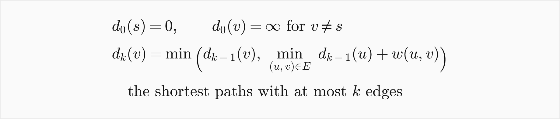
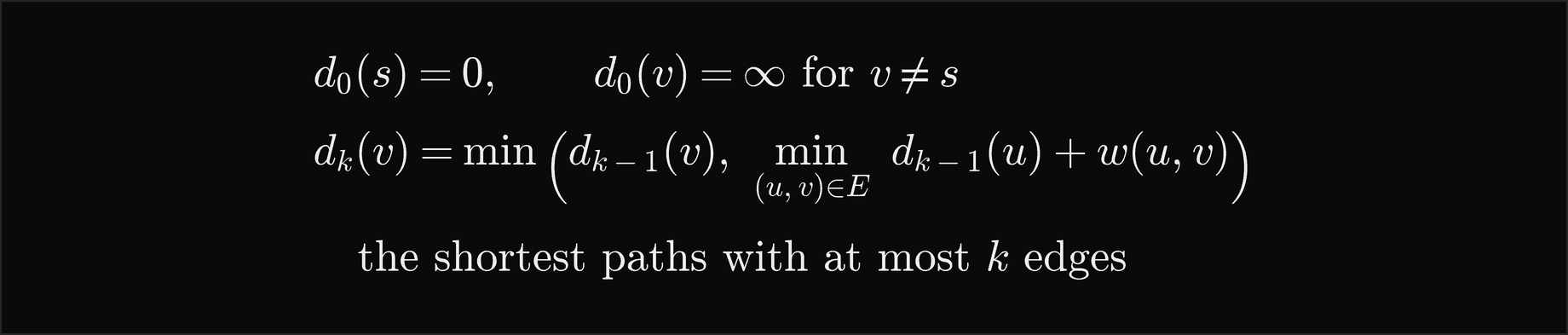
d 0 of s is 0 and d 0 of v is infinity for v other than s; d k of v is the minimum of d k minus 1 of v and, over all edges u to v, d k minus 1 of u plus the weight of u to v: the shortest paths with at most k edges

The package implements both readings. The synchronous version reads every tail's distance from the end of the previous pass, so after pass k it holds exactly d_k, whatever the edge order. The usual in-place version uses distances already lowered earlier in the same pass, so a good edge order can carry a value along a whole path in one pass, and after pass k it is at least as far along:

delta of s and v is at most d of v, which is at most d k of v, after pass k of the in-place version

The final distances never depend on the order of the edges; the intermediate tables do. A table of d[v] after each pass is only meaningful together with the edge order it was computed in, which is why the worked example lists its order first. When nothing changes in a whole pass, no edge is tense, and nothing will ever change again: the algorithm can stop early. The number of passes is then at most L + 1, where L is the largest number of edges on any shortest path from s.

Negative cycles¶

A negative cycle reachable from s drags the distance of everything it can reach down to −∞:

The weight of a cycle c from v0 back to v k equal to v0 is the sum of its edge weights; if it is negative, delta of s and v is minus infinity for every v reachable from c

Bellman-Ford detects one with a single extra pass. Without a reachable negative cycle, all distances are final after n − 1 passes and the check pass changes nothing. With one, some edge of the cycle is always tense, and the check pass changes something. Suppose instead that no edge of a reachable negative cycle c = ⟨v0, v1, ..., vk = v0⟩ were tense; adding the k inequalities around the cycle, the distances cancel because every vertex appears once on each side, and what remains contradicts the cycle's negative weight:

If no edge of c is tense, then d of v i is at most d of v i minus 1 plus the weight of the edge, for i from 1 to k; summing, the sum of d of v i is at most the sum of d of v i minus 1 plus w of c, so 0 is at most w of c

The parents left behind point the way to the cycle. Take a vertex whose distance dropped in the check pass and follow its parents. The chain ends up circling a cycle of parents, and every cycle of parents has negative weight, but it may first pass through vertices that only hang off the cycle. Walking back n steps first is always enough to be on the cycle; from there, extract_negative_cycle collects vertices until the walk comes round again and reverses them into edge direction. find_negative_cycle finds a negative cycle anywhere, reachable from a given source or not, by adding an imaginary source joined to every vertex by an edge of weight 0. reachable_from lists the vertices whose distance is −∞.

Two applications explain why detection matters as much as distances. In currency exchange, an edge weight of −log(rate) turns a sequence of exchanges whose rates multiply to more than 1 into a negative cycle, an arbitrage opportunity. And in an undirected graph a single negative edge is already a negative cycle of two edges, u→v→u, so Bellman-Ford on undirected graphs with negative weights always reports a cycle; such graphs need different methods.

Directed acyclic graphs¶

A graph without cycles has a topological order, an order of its vertices in which every edge points forward (see Topological sorting). Every path visits its vertices in that order, so relaxing the out-edges of each vertex in topological order relaxes the edges of every shortest path in path order, and path relaxation makes every distance final after one relaxation per edge. Negative weights are fine, because there are no cycles to be negative. The package finds the order with Kahn's algorithm, taking vertices that become ready at the same time in insertion order, so the trace is deterministic. Vertices before the source in the order cannot be reached from it; relaxing their edges offers ∞ and changes nothing. Negating every weight turns the same algorithm into a longest-path algorithm, dag_longest_paths, which finds the critical path of a project plan: the chain of dependent tasks that decides the earliest finish. On a graph with cycles, longest simple paths are NP-hard.

Fewest edges: breadth-first search¶

When every edge costs the same, the priority queue is unnecessary. A first-in first-out queue holds vertices at distance k followed by vertices at distance k + 1 and nothing else, so it hands them out in order of distance just as the heap would, each vertex is settled the first time it is reached, and each edge is relaxed once. That is breadth-first search, fewest_edges, covered in depth in Breadth-first and depth-first search. The sample project uses it to find itineraries with the fewest flights.

A* search¶

For one target t, Dijkstra explores in every direction, settling every vertex closer to s than t is. A* orders the queue by the cost so far plus a guess of the cost still to go:

f of v equals g of v plus h of v

Here g(v) is the tentative distance from s, Dijkstra's key, and h(v) is a heuristic estimate of the distance from v to t. With h = 0, A* is Dijkstra. A heuristic is admissible when it never overestimates:

h of v is at most delta of v and t, for every vertex v

and consistent when it obeys the triangle inequality along every edge and is 0 at the target. Consistency implies admissibility, by adding the inequalities along a shortest path to t:

h of u is at most the weight of u to v plus h of v for every edge, and h of t is 0; therefore h of v0 is at most w of v0 v1 plus h of v1, and so on, up to w of p plus h of t, which equals delta of v0 and t, along a shortest path p to t

With a consistent heuristic, A* is Dijkstra's algorithm on reduced weights. Each reduced weight is at least zero exactly because of consistency, and along any path the reductions telescope, changing every path from s to v by the same amount, so shortest paths stay shortest:

The reduced weight w h of u and v equals w of u and v minus h of u plus h of v, which is at least zero; the reduced weight of a path p from s to v equals w of p minus h of s plus h of v

The reduced distance of v is g(v) − h(s) + h(v), which is f(v) up to the constant h(s), so Dijkstra on reduced weights takes vertices in order of f, exactly as A does. Everything proved for Dijkstra carries over: each vertex is expanded at most once, the target leaves the queue with its correct distance, and the search must stop when the target is expanded, not when it is first reached. With an admissible but inconsistent heuristic, a cheaper path to an expanded vertex can still turn up; the package's astar then reopens the vertex and expands it again, and the answer stays optimal. An overestimating heuristic gives no guarantee: multiplying an admissible h by a factor of 2, weighted A, usually expands fewer vertices but can return a path up to twice as long as the shortest.

On a grid where a move to one of the four neighbours costs 1, the Manhattan distance is the classic consistent heuristic: no path can be shorter than the rows plus the columns between two cells, and one move changes that count by exactly 1.

h of a cell at row r and column c equals the absolute difference of r and the target's row plus the absolute difference of c and the target's column

The figure below compares it with no heuristic and with the straight-line distance on a grid with a wall between the start and the goal.

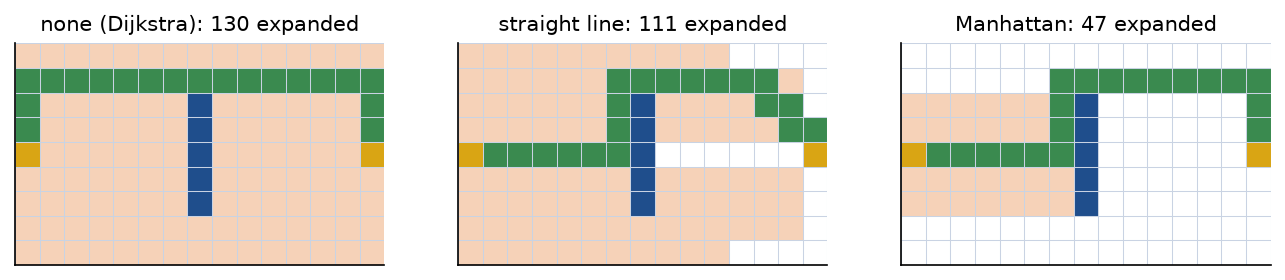
Three panels of the same 9 by 15 grid with a wall of five cells between the start on the left and the goal on the right: with no heuristic 130 cells are expanded, all of the free cells; with the straight-line distance 111; with the Manhattan distance only 47, most of them on the start's side of the wall; the green path has 20 moves in every panel

The figure, written by examples/astar_on_grids.py, shows the expanded cells in pale orange. Without a heuristic the search fills the whole grid, because 130 free cells are closer to the start than the goal at distance 20 is, or as close. The straight-line distance is consistent too, but it is smaller than the Manhattan distance and guides the search less. Every cell whose g + h is below 20 must be expanded by any A* with the Manhattan heuristic, 35 cells here; 65 more cells have g + h exactly 20, and which of those are expanded depends on how ties are broken. The package breaks ties between equal f in favour of the smaller h, the vertex nearer the target, and expands only 12 of them; Dijkstra on the reduced weights, which follows the same f order with an arbitrary tie rule, settles 83 cells in all.

Reading paths from parent pointers¶

A shortest path is read backwards: start at the target, follow parents until the source, and reverse the walk. path_to returns None for an unreached vertex, whose parent is None, and raises an error if the walk grows longer than the number of vertices, which only happens when a negative cycle has bent the parents into a loop. The source has no parent, which the package records as None; code that marks "no parent" with 0, or tests a parent with while parent[v]:, silently cuts paths short at a vertex called 0. When filling a table by hand, the parent of v is the tail of the last edge that lowered d[v], not the vertex extracted just before v.

Cost¶

Every algorithm¶

For a graph with n vertices and m edges, all reachable from the source, Dijkstra with a binary heap makes n pushes and n pops, each O(log n), and at most m decrease-keys, each O(log n). Every edge is relaxed exactly once:

T is n times the cost of a push plus n times the cost of a pop plus m times the cost of a decrease-key; with a binary heap each is O of log n, so T is O of n plus m, times log n

With a plain list instead of a heap, the scans make exactly n(n − 1)/2 comparisons, and the whole run is Θ(n²), which is the best possible for a dense graph:

The comparisons are the sum over k from 1 to n of k minus 1, which is n times n minus 1 over 2; T is n times Theta of n plus m times O of 1, which is Theta of n squared

A Fibonacci heap makes decrease-key O(1) amortized, which gives the classic bound for sparse graphs in theory, although in practice binary and 4-ary heaps win on constant factors:

n times O of log n plus m times O of 1 is O of m plus n log n, amortized, with a Fibonacci heap

Lazy deletion keeps up to one heap entry per improvement, so the heap can grow to m + 1 entries; the time is still O(m log n), with O(m) extra space:

The heap holds at most m plus 1 entries, and O of m log m equals O of m log n, since log m is less than 2 log n

Bellman-Ford relaxes all m edges in each pass and runs at most n passes including the check; with early stopping it runs L + 1:

L is the largest number of edges on a shortest path to any vertex, at most n minus 1; T is the number of passes times m, at most L plus 1 times m, at most n times m, which is O of n m

The DAG algorithm and breadth-first search look at every vertex and every edge once, which no algorithm can avoid:

T is Theta of n plus m: one topological sort, then one relaxation per edge

A* costs, in the worst case, with an uninformative heuristic, what Dijkstra costs; how much less it does depends entirely on the heuristic, as the measurements below show.

All of these are worst-case bounds, except the Fibonacci heap's, which is amortized: a single decrease-key can still be slow, but any sequence of them is cheap on average. Space is O(n + m) for the graph and O(n) for distances, parents and the indexed heap.

Counted comparisons: heap against list¶

The example relaxation_costs.py counts the queue comparisons of the three Dijkstras on random sparse graphs with m = 4n, and the total work, relaxations plus comparisons plus swaps, on the complete DAG in which every edge lowers a distance, the worst case for decrease-keys. The bound for the heap is the counted pops, pushes and decrease-keys, each multiplied by its cost per level:

The comparisons are at most two times the pops plus the pushes plus the decrease-keys, times the floor of log base 2 of n

The left panel draws this bound over the measured comparisons; the right panel shows the dense worst case.

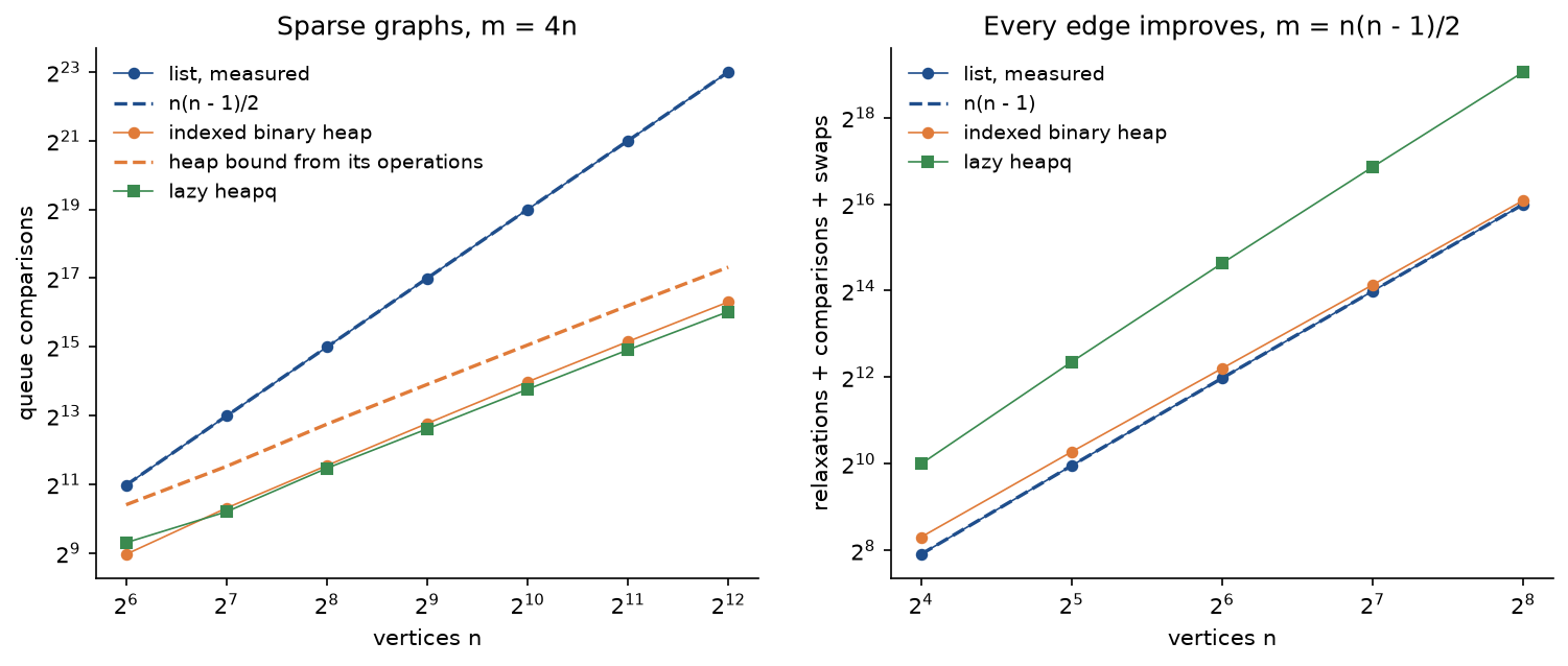
On sparse graphs the heap wins by a widening margin: at n = 4096 the list makes 8386560 comparisons, exactly n(n − 1)/2, against 81072 for the indexed heap, under its bound of 163476, and 66694 for lazy heapq. Only 1335 of the 16384 edges triggered a decrease-key; on random graphs most relaxations fail, which is why the classical bound, which charges every edge a decrease-key, is far from the measured cost. On the dense worst case every one of the n(n − 1)/2 edges improves a distance, and the picture turns round: at n = 256 the list does 65280 operations, exactly n(n − 1), against 69514 for the indexed heap, which makes 32385 decrease-keys, and 544085 for lazy heapq, whose heap grows to one entry per edge. On dense graphs the plain list is as good as any heap, and simpler.

Relaxations by algorithm¶

The same random graphs measure how many relaxations each algorithm needs.

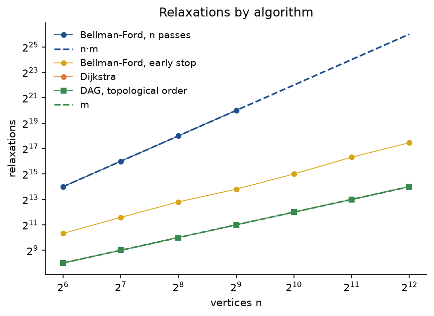
A log-log plot of relaxations against n from 64 to 4096 on graphs with m equal to 4n: Bellman-Ford with all n passes lies on the dashed n times m line, measured up to n equal to 512; Bellman-Ford with early stopping grows a little faster than m, reaching 180 thousand at 4096; Dijkstra and the DAG algorithm both lie exactly on the dashed line m

Dijkstra and the DAG algorithm, on random DAGs of the same size, relax exactly m edges, 16384 at n = 4096. The textbook Bellman-Ford relaxes n·m, 67108864 at that size; it was measured up to n = 512, where it agrees exactly. Early stopping changes everything on random graphs: shortest paths there have few edges, so 11 passes sufficed at n = 4096, 180224 relaxations, eleven times Dijkstra's count rather than four thousand times. It is no help in the worst case: on a path whose edges are listed from the far end back, each pass carries the distances one edge further and all n passes are needed, which backward_path builds and the tests check.

What a heuristic saves¶

The example astar_on_grids.py runs A* on random grids with a quarter of the cells walls, the start and the goal in opposite corners, five grids per size, and counts expanded cells.

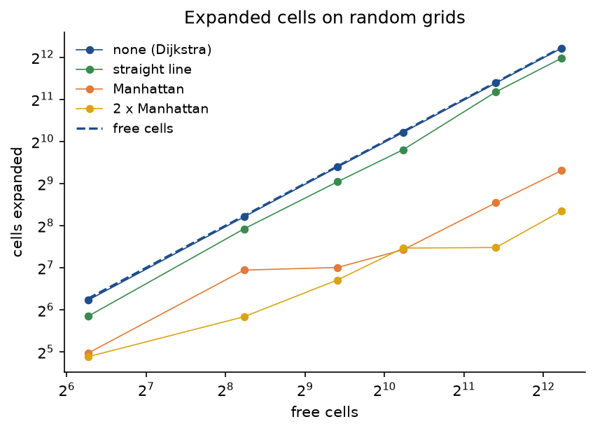
A log-log plot of expanded cells against the number of free cells, from about 77 to about 4800: without a heuristic the search expands almost every free cell and lies on the dashed line of free cells; the straight-line heuristic saves 13 to 25 percent; the Manhattan heuristic expands far fewer, about 634 of 4792 at the largest size; twice the Manhattan distance expands fewer still

On 80 by 80 grids, with 4791.6 free cells on average, Dijkstra expanded 4748.2 cells, A with the straight-line distance 4027.6 and A with the Manhattan distance 633.6, all three returning the same path length. Twice the Manhattan distance expanded 325.6, but it overestimates, and on 26 of the 30 grids it returned a path longer than the shortest, by a factor of up to 1.2222. A heuristic closer to the true cost to go expands fewer vertices; one that is too close, overestimating, gives up the guarantee.

Worked example¶

Every step below is printed by examples/worked_example.py and asserted by tests/test_worked_example.py.

Dijkstra step by step¶

The graph has the vertices S, A, B, C, D and E and ten edges, listed with each vertex's out-edges in the order they are relaxed: S→B 8, S→E 1, A→B 6, A→D 4, B→A 6, B→C 8, B→D 2, D→C 4, E→A 3, E→B 4. The source is S. Each bullet extracts the vertex with the smallest key, relaxes its out-edges, and ends with the table of distances and parents:

Extract S (0). S→B: 0 + 8 = 8 < ∞, push B. S→E: 0 + 1 = 1 < ∞, push E. Table: S 0, A ∞, B 8 via S, C ∞, D ∞, E 1 via S.
Extract E (1); the queue held E 1 and B 8. E→A: 1 + 3 = 4 < ∞, push A. E→B: 1 + 4 = 5 < 8, decrease B's key to 5, parent E. Table: S 0, A 4 via E, B 5 via E, C ∞, D ∞, E 1 via S.
Extract A (4); the queue held A 4 and B 5. A→B: 4 + 6 = 10 ≥ 5, no change. A→D: 4 + 4 = 8 < ∞, push D. Table: S 0, A 4 via E, B 5 via E, C ∞, D 8 via A, E 1 via S.
Extract B (5); the queue held B 5 and D 8. B→A: 5 + 6 = 11 ≥ 4, no change, and A is settled anyway. B→C: 5 + 8 = 13 < ∞, push C. B→D: 5 + 2 = 7 < 8, decrease D's key to 7, parent B. Table: S 0, A 4 via E, B 5 via E, C 13 via B, D 7 via B, E 1 via S.
Extract D (7); the queue held D 7 and C 13. D→C: 7 + 4 = 11 < 13, decrease C's key to 11, parent D. Table: S 0, A 4 via E, B 5 via E, C 11 via D, D 7 via B, E 1 via S.
Extract C (11). It has no out-edges, and the queue is empty.

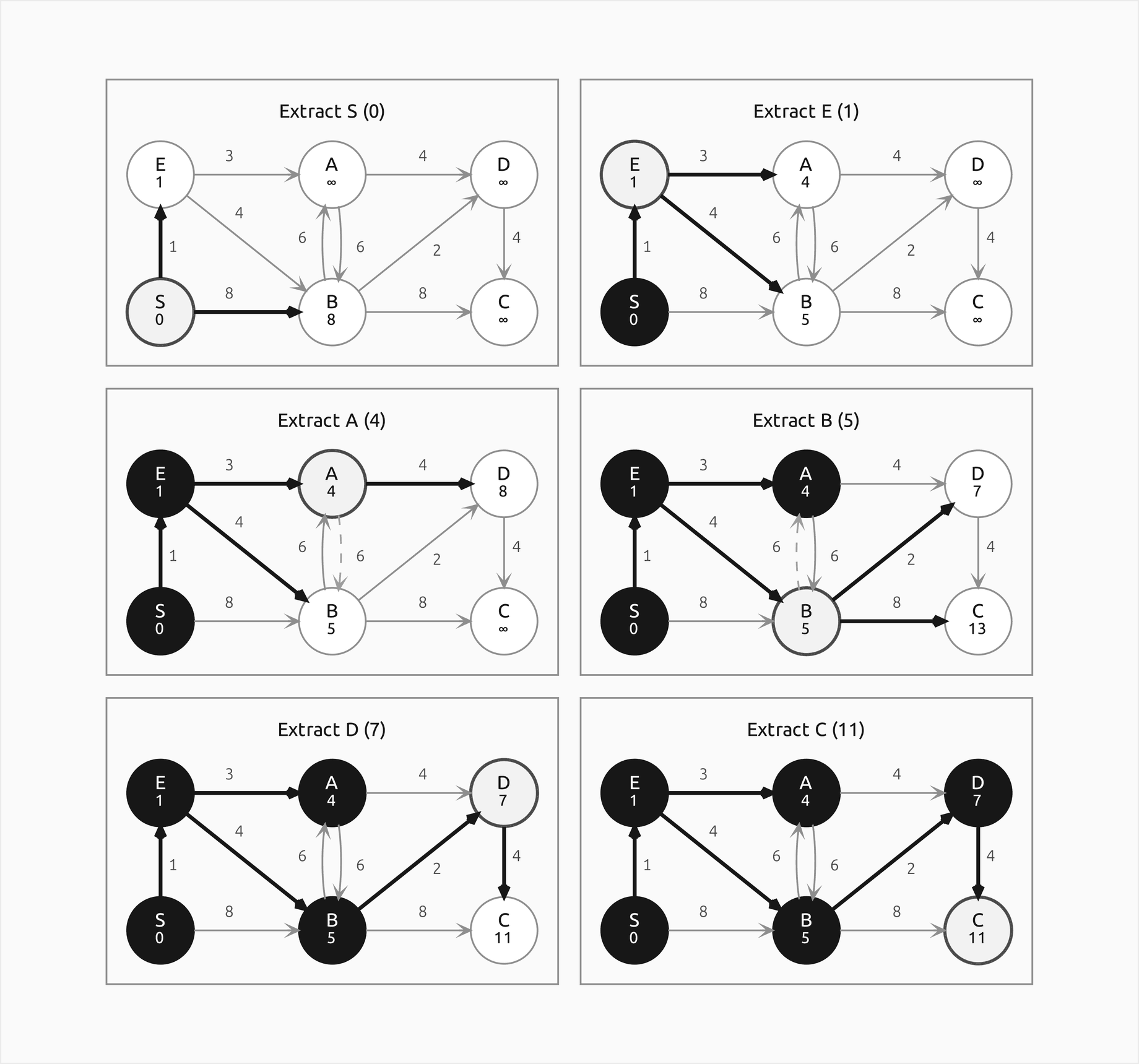
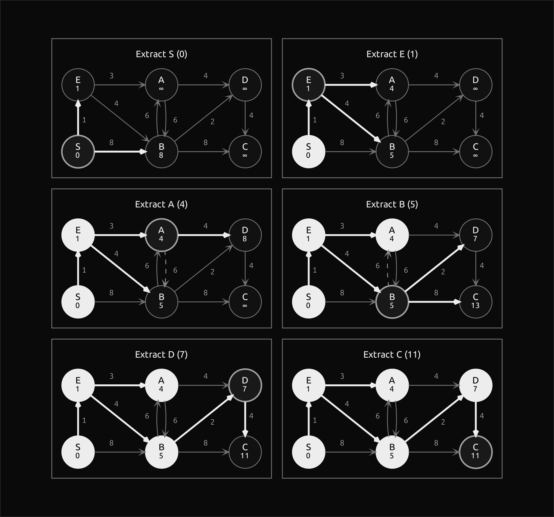
Each frame shows the state after an extraction and the relaxations that follow it. Three distances dropped after they were first set, B from 8 to 5, D from 8 to 7 and C from 13 to 11, and each drop moved a bold tree edge. Two relaxations changed nothing: A→B, because B already had 5, and B→A, into a settled vertex.

The extraction order is S, E, A, B, D, C, with nondecreasing keys 0, 1, 4, 5, 7, 11. The paths read from the parents are S→E→A (4), S→E→B (5), S→E→B→D (7) and S→E→B→D→C (11): to read C's path, walk C, D, B, E, S and reverse. The run made 10 relaxations, 8 of which improved a distance, 6 pushes, 6 pops and 3 decrease-keys, and the indexed heap made 5 comparisons and 6 swaps. The lazy version on heapq made 9 pushes and 9 pops, of which 3 were stale entries left behind by the three decreases: B with key 8, D with key 8 and C with key 13.

Bellman-Ford pass by pass¶

The graph has the vertices S, M, N, P, Q and R, the source S, two negative edges and no negative cycle. Each pass relaxes the ten edges in this order: M→P 2, M→Q 7, N→M −3, N→P 5, P→Q −2, P→R 2, Q→R 5, R→N 2, S→M 6, S→N 4. Only the relaxations that change something are listed:

Pass 1. Every edge before S→M starts at a vertex still at ∞. S→M: M = 6 via S. S→N: N = 4 via S. After the pass: S 0, M 6 via S, N 4 via S, P ∞, Q ∞, R ∞.
Pass 2. M→P: 6 + 2 = 8, P = 8 via M. M→Q: 6 + 7 = 13, Q = 13 via M. N→M: 4 − 3 = 1 < 6, M = 1 via N. P→Q: 8 − 2 = 6 < 13, Q = 6 via P. P→R: 8 + 2 = 10, R = 10 via P. After the pass: S 0, M 1 via N, N 4 via S, P 8 via M, Q 6 via P, R 10 via P.
Pass 3. M→P: 1 + 2 = 3 < 8, P = 3 via M. P→Q: 3 − 2 = 1 < 6, Q = 1 via P. P→R: 3 + 2 = 5 < 10, R = 5 via P. After the pass: S 0, M 1 via N, N 4 via S, P 3 via M, Q 1 via P, R 5 via P.
Pass 4. Nothing changes, so the run stops after 4 passes and 40 relaxations instead of 5 passes and a check, 60 relaxations.

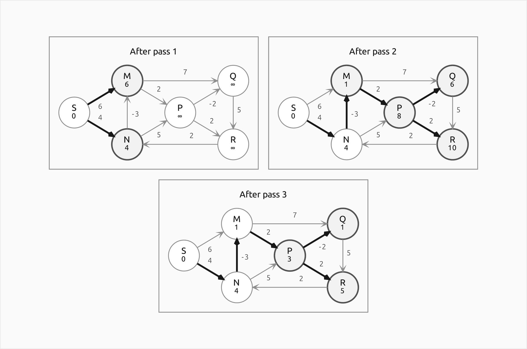
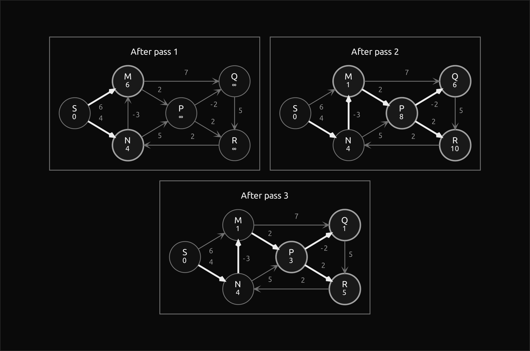
The first pass did little because the edges out of S come last in the order. Relaxing the edges along the shortest paths instead, S→M, S→N, N→M, N→P, M→P, M→Q, P→Q, P→R, Q→R, R→N, makes every distance final in the first pass, and the second pass, which changes nothing, ends the run after 2 passes. The synchronous version needs 5 passes, one per edge of the longest shortest path S→N→M→P→Q plus a quiet one; its table after pass 2 is S 0, M 1 via N, N 4 via S, P 8 via M, Q 13 via M, R ∞, the shortest paths with at most two edges, while the in-place version had already reached Q = 6 and R = 10. All three orders end with the same distances: M 1, N 4, P 3, Q 1, R 5.

A negative cycle¶

Lowering R→N from 2 to −2 closes the cycle N→M→P→R→N of weight −3 + 2 + 2 − 2 = −1. The passes never settle down: after pass 5 the distances are S 0, M 0, N 2, P 2, Q 0, R 4, and the check pass, pass 6, still lowers M to −1 via N. To extract the cycle, start at M and walk back six parents, through N, R, P, M, N to R, which is certainly on the cycle; collecting from R gives R, P, M, N before the walk returns to R, and reversing gives the cycle N→M→P→R→N.

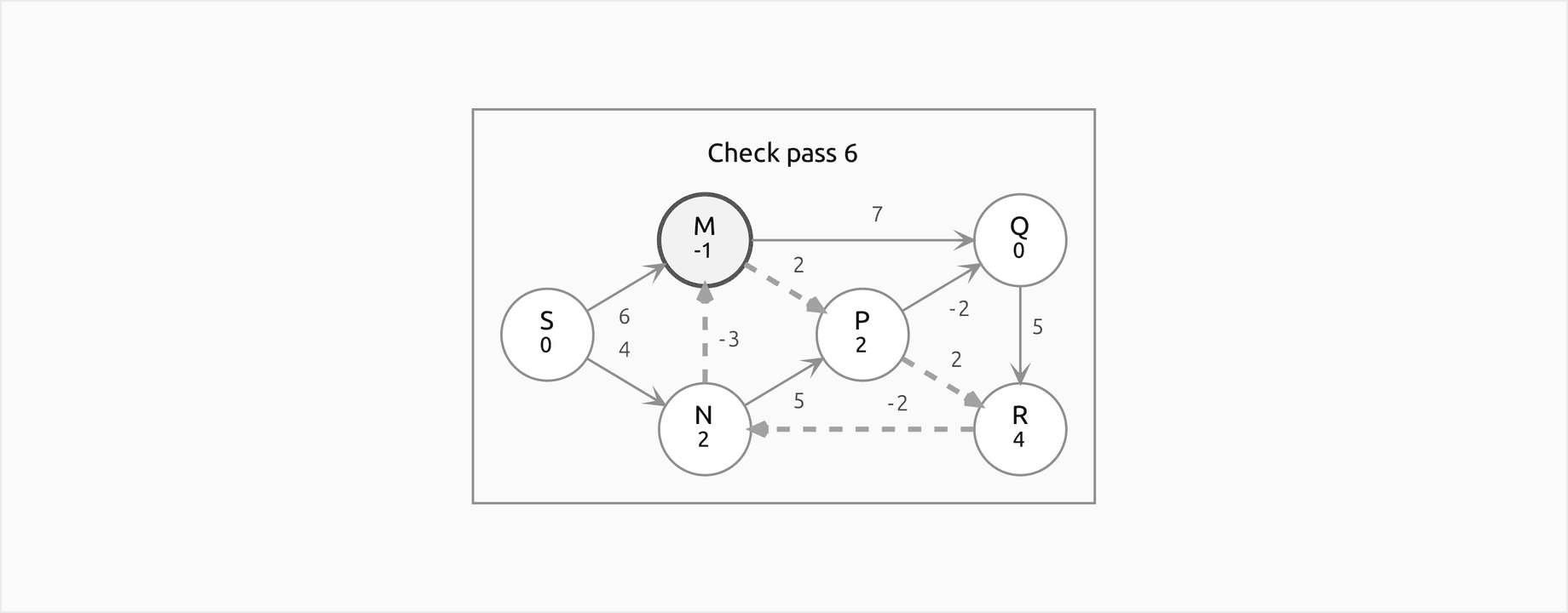
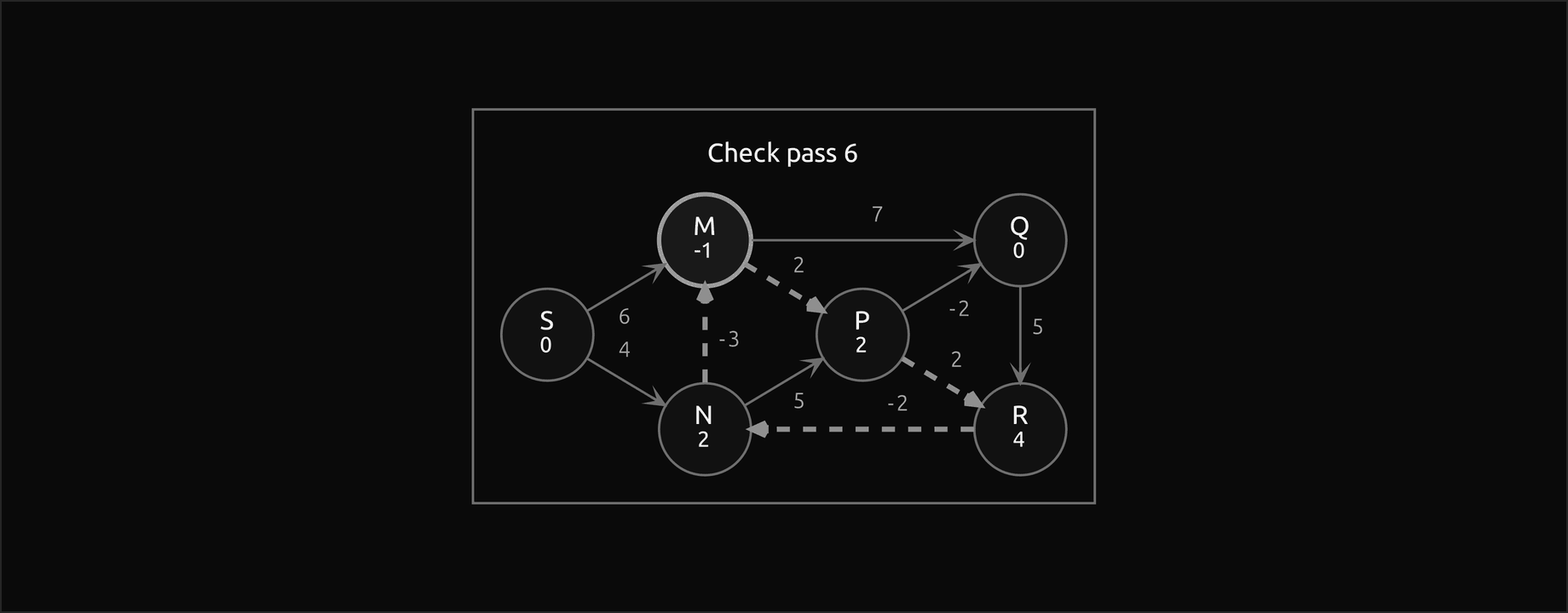
The same graph with R to N lowered to minus 2, after the check pass: the cycle N to M to P to R and back is dashed and bold, with its weights minus 3, 2, 2 and minus 2, M is outlined because it still changed, and the vertices show the distances after six passes

Every vertex reachable from the cycle, M, N, P, Q and R, has distance −∞; only S keeps a real distance. The tempting shortcut of following parents from a vertex that changed, without the n steps back, can collect a vertex that hangs off the cycle: started at Q, it returns R, N, M, P, Q, which includes Q although Q is not on the cycle.

A DAG in topological order¶

The DAG has the vertices Z, S, A, B, C, D and T and eleven edges, two of them negative: Z→S 2, Z→A 1, S→A 4, S→B 6, S→D 3, A→B −3, A→C 5, B→C 2, B→T 7, C→T −1, D→T 4. Kahn's algorithm gives the order Z, S, A, D, B, C, T, and the source is S:

Z is at ∞, so Z→S and Z→A change nothing.
S (0): A = 4, B = 6 and D = 3, all via S.
A (4): A→B gives 4 − 3 = 1 < 6, B = 1 via A; A→C gives C = 9 via A.
D (3): D→T gives T = 7 via D.
B (1): B→C gives 3 < 9, C = 3 via B; B→T gives 8 ≥ 7, no change.
C (3): C→T gives 3 − 1 = 2 < 7, T = 2 via C.
T (2) has no out-edges.

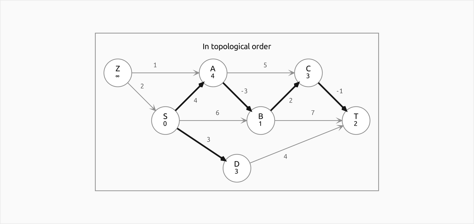
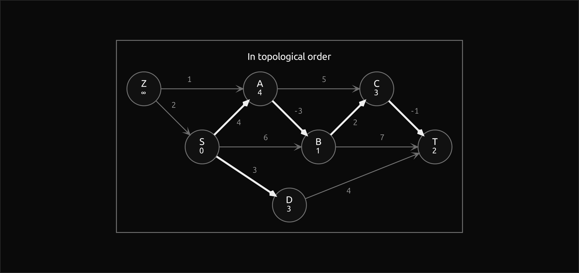
The DAG laid out from left to right in the topological order Z, S, A, D, B, C, T, with Z, A and C in the top row, S, B and T in the middle row and D alone below, so every edge points right; the final distances are Z infinity, S 0, A 4, D 3, B 1, C 3 and T 2, and the tree edges S to A, A to B, B to C, C to T and S to D are bold The DAG laid out from left to right in the topological order Z, S, A, D, B, C, T, with Z, A and C in the top row, S, B and T in the middle row and D alone below, so every edge points right; the final distances are Z infinity, S 0, A 4, D 3, B 1, C 3 and T 2, and the tree edges S to A, A to B, B to C, C to T and S to D are bold

Eleven relaxations, one per edge, eight of which improved a distance, find every distance. The shortest path to T is S→A→B→C→T with weight 4 − 3 + 2 − 1 = 2, which uses both negative edges, and Z, which comes before the source, stays unreached.

The code¶

The package shortest_paths is plain Python, one idea per module. Importing it needs only the standard library and the heaps topic's package; Matplotlib is imported by plotting.py alone, and NetworkX and SciPy inside the functions of comparisons.py.

graph.py holds Edge and WeightedDigraph, the small graph class every algorithm reads.
counting.py holds OperationCounter, with the fields relaxations, improvements, pushes, pops, decreases, comparisons and swaps, which every algorithm accepts as an optional counter, and CountedKey, which counts the comparisons heapq makes.
trace.py holds the Step record, record, annotate and the text forms printed above: describe, format_trace, format_state and format_cell.
relaxation.py holds initialize_single_source, relax and is_tense; paths.py holds ShortestPaths, the result of every single-source run, and path_to, path_weight and tree_edges.
dijkstra.py holds dijkstra on the indexed heap, lazy.py holds dijkstra_lazy on heapq and dense.py holds dijkstra_array with a plain list.
bellman_ford.py holds bellman_ford, in place or synchronous, with early stopping and a pass limit, and negative_cycles.py holds extract_negative_cycle, cycle_weight, find_negative_cycle and reachable_from.
dag.py holds topological_order, dag_shortest_paths and dag_longest_paths; unweighted.py holds fewest_edges.
astar.py holds astar, heuristics.py the checks is_admissible and is_consistent with reduced_graph and scaled, and grids.py the grid worlds with manhattan and euclidean.
invariants.py holds the certificate check shortest_paths_violation with check_shortest_paths, upper_bound_violation and graph_violation; oracle.py holds brute_force_distances, which tries every simple path of a tiny graph.
workloads.py holds the worked examples and seeded random graphs: general, with negative weights but no negative cycle, with a planted negative cycle, acyclic, the backward path and the graph on which every edge improves.
drawing.py returns deterministic Graphviz text for one or several states of a run, every vertex pinned at the same place in every frame; layout.py holds the place of every vertex of the worked graphs, spreads any other graph round a circle and sizes the frames and their rows; comparisons.py puts NetworkX and SciPy next to the package; pitfalls.py holds deliberately broken versions for the pitfalls below; plotting.py draws every figure in the handbook's colours.

The examples run in a few seconds each from the repository root:

examples/worked_example.py prints every step of the worked example and writes the five generated diagram sources.
examples/relaxation_costs.py counts comparisons and relaxations for the cost section.
examples/astar_on_grids.py compares A* with Dijkstra on grids and checks the reduced-weight view.
examples/common_mistakes.py runs every broken version from pitfalls.py next to the correct code.
examples/compare_with_libraries.py checks the package against NetworkX and SciPy and times them roughly.
examples/practice.py prints fresh exercises with their solutions; --seed gives a new set.

python graphs/shortest-paths/examples/worked_example.py
python graphs/shortest-paths/examples/relaxation_costs.py
python graphs/shortest-paths/examples/astar_on_grids.py
python graphs/shortest-paths/examples/common_mistakes.py
python graphs/shortest-paths/examples/compare_with_libraries.py
python graphs/shortest-paths/examples/practice.py --seed 7

The sample project, project/route_planner.py with its helpers project/openflights.py and project/geography.py, plans itineraries on the world's airline network. On first use it downloads the OpenFlights airports and routes files, pinned to one commit of the OpenFlights repository and checked against SHA-256 checksums, into .data/shortest-paths/ at the repository root. Every pair of airports joined by a direct route becomes an edge, 36707 of them between 3193 airports, weighted by the great-circle distance in kilometres, computed with the haversine formula:

a is the sine squared of half the difference in latitude, plus the cosine of the first latitude times the cosine of the second times the sine squared of half the difference in longitude; d is 2R times the arcsine of the square root of a, with R equal to 6371.0088 km

For each origin and destination the project finds the itinerary with the fewest flights, the shortest one, the shortest with at most k flights, and A* against Dijkstra. Fewest flights, with ties broken by distance, is Dijkstra with a large penalty per flight, larger than any itinerary is long, so that one flight fewer always wins:

The cost of an itinerary p is M times its number of flights plus its length in km, with M equal to one million, more than the length of any itinerary

The shortest itinerary with at most k flights is exactly the synchronous Bellman-Ford after k passes. And the great-circle distance to the destination is a consistent A* heuristic, because distances on a sphere obey the triangle inequality and every edge weight is itself a great-circle distance. The default run takes under ten seconds:

Cape Town to Lima, 9781 km apart: the fewest flights are 2, CPT→AMS→LIM, 20207 km by way of Amsterdam; the shortest itinerary is CPT→JNB→GRU→LIM, 12185 km in 3 flights. Dijkstra settled 1572 airports before Lima, A* only 17.
Perth to Fairbanks: 3 flights by way of Dubai and Seattle, 23431 km, against 4 flights by way of Brisbane, Honolulu and Anchorage, 16053 km.
Ushuaia to Cape Town: 3 flights by way of Buenos Aires and London, 23168 km, against 4 by way of Buenos Aires, São Paulo and Johannesburg, 12783 km. With at most 3 flights the best is 23168 km; a fourth flight saves 10385 km.

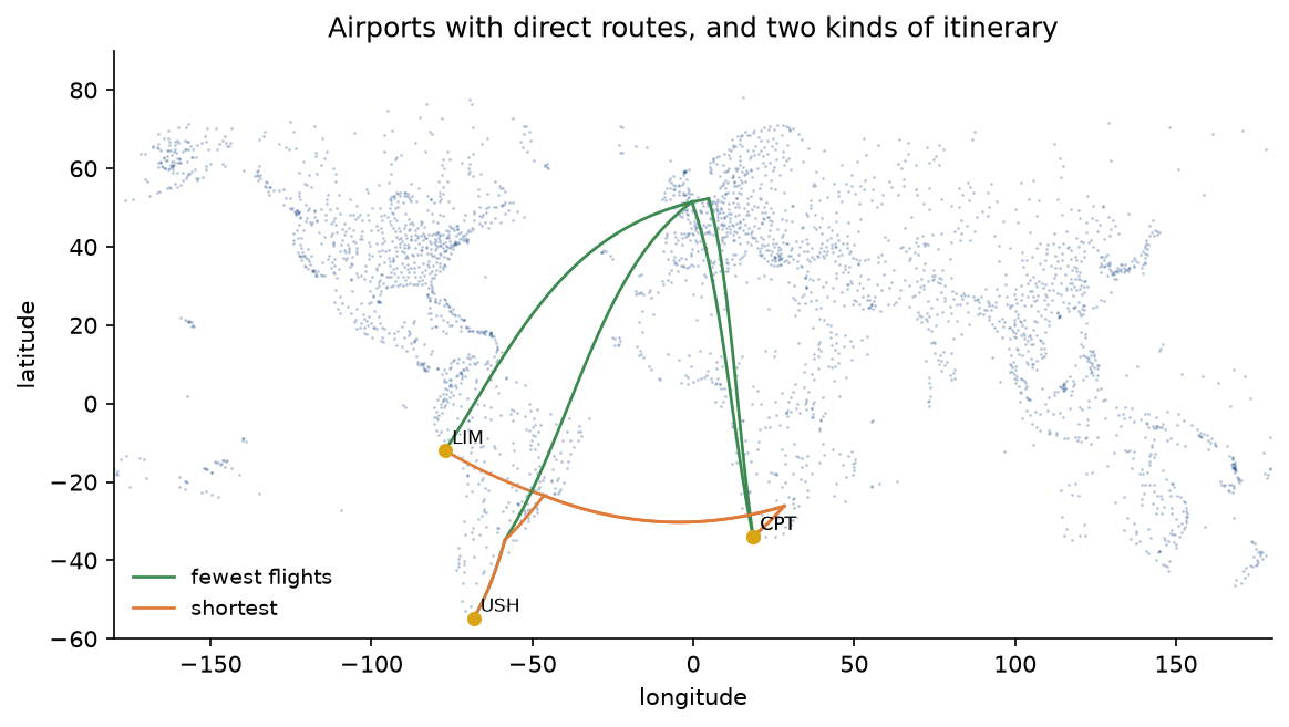
A world map of the 3193 airports with direct routes, as pale dots, with two pairs of itineraries drawn along great circles: from Cape Town to Lima and from Ushuaia to Cape Town, the fewest-flight itineraries in green both detour through Europe, while the shortest itineraries in orange cross the South Atlantic by way of Johannesburg and São Paulo

The map shows why the two questions have different answers: the fewest flights go through a hub in Europe, while the shortest route stays in the southern hemisphere and pays for it with an extra flight.

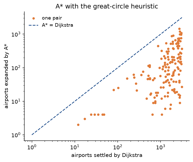
A log-log scatter of 150 random reachable pairs of airports: the number of airports A* expanded against the number Dijkstra settled before reaching the destination; every point lies below the dashed diagonal, most of them one or two orders of magnitude below

Over 150 random reachable pairs, A* expanded on average 0.1192 of the airports Dijkstra settled, with a median of 0.0825, and every length agreed. The run also checks the distances and the fewest flights from five random airports against NetworkX. Options --routes (pairs such as CPT-LIM,PER-FAI), --pairs, --max-flights, --checks and --seed change the questions, --data the download folder and --figures where the PNGs go.

python graphs/shortest-paths/project/route_planner.py
python graphs/shortest-paths/project/route_planner.py --routes HNL-CPT,KEF-AKL --pairs 50

The OpenFlights airport and route databases are made available under the Open Database License (ODbL 1.0), with their individual contents under the Database Contents License; this page's map and statistics are derived from them. Nothing is committed: the files live in the git-ignored .data folder. All other data on this page are synthetic, generated from seeds by workloads.py.

The notebook shortest_paths.ipynb follows this page: the worked examples step by step, the diagrams, the negative edge and the negative cycle, A* on a grid, the counted costs, the comparisons with NetworkX and SciPy and the project's route planner on two airports. The tests in tests check the worked examples value by value, the certificate on the answers for about a hundred random graphs, the upper-bound property at every step of seeded runs, the counts the cost section relies on, every pitfall, and the agreement with a brute-force oracle, NetworkX and SciPy, and run in a few seconds:

python -m pytest graphs/shortest-paths

In practice¶

NetworkX and SciPy¶

NetworkX computes single-source shortest paths with single_source_dijkstra_path_length, single_source_bellman_ford_path_length, single_source_shortest_path_length (breadth-first search) and astar_path_length, and finds negative cycles with find_negative_cycle. scipy.sparse.csgraph.shortest_path takes a sparse matrix and a method: "D" for Dijkstra, "BF" for Bellman-Ford and "J" for Johnson's algorithm. examples/compare_with_libraries.py checks that they agree with the package:

from shortest_paths import dijkstra, random_digraph
from shortest_paths.comparisons import networkx_dijkstra, scipy_distances

graph = random_digraph(200, 900, seed=1)
ours = dijkstra(graph, 0).distance
reached = {vertex: d for vertex, d in ours.items() if d != float("inf")}
assert reached == networkx_dijkstra(graph, 0)
assert ours == scipy_distances(graph, 0, "D")

The distances agree on every random graph tried, including graphs with negative edges for Bellman-Ford and Johnson, and NetworkX's A* returns the same lengths on grids. The libraries differ in how they treat bad input. On the four-vertex negative-edge graph, NetworkX's Dijkstra raises ValueError with the message "Contradictory paths found: negative weights?", while SciPy's warns that "dijkstra will give inaccurate results if the graph contains negative cycles" and returns an answer, which happens to be right on this small graph but comes with no guarantee. NetworkX leaves unreachable vertices out of its result instead of reporting infinity.

Building the sparse matrix for SciPy has two traps. Converting a list of (row, column, weight) triples to a matrix adds up duplicate entries, so two parallel edges of weights 5 and 3 become one edge of weight 8; to_csr keeps the lighter one instead. And in a dense matrix a 0 means "no edge", while in a sparse matrix an explicitly stored 0 is an edge of weight 0. In rough wall-clock terms, NetworkX's Dijkstra ran about 5 times as fast as the package's on 20000 vertices and 100000 edges, and SciPy's roughly 80 times, the usual gap between pure Python, Python with lighter bookkeeping, and compiled code.

When to use which:

Use breadth-first search when every edge costs the same.
Use Dijkstra with a binary heap for weights of at least zero; in Python, heapq with lazy deletion is the usual choice, and an indexed heap pays off when memory matters or decrease-keys are many.
Use a plain list instead of a heap when the graph is dense, with m close to n².
Use the DAG algorithm whenever the graph has no cycles, including for longest paths and with negative weights.
Use Bellman-Ford when weights can be negative, with early stopping, and when negative cycles must be detected or found.
Use A* for one target when a consistent lower bound on the remaining cost is at hand, such as a straight-line or great-circle distance.
Use SciPy's csgraph for large graphs held as matrices, and NetworkX when convenience and a rich graph model matter more than speed.

Elsewhere¶

Link-state routing protocols such as OSPF and IS-IS run Dijkstra on every router over the whole network map, while distance-vector protocols such as RIP are Bellman-Ford spread over the routers, each relaxing the edges to its neighbours, and BGP extends that idea with whole paths. Road navigation services cannot afford a Dijkstra over a continent per query; they precompute shortcuts with contraction hierarchies, run bidirectional searches that meet in the middle, or use A* with landmark-based lower bounds (ALT), and answer queries in milliseconds. Integer weights in a small range allow bucket queues (Dial's algorithm) and radix heaps instead of comparison heaps. C++ programs usually write Dijkstra with std::priority_queue and lazy deletion, the Boost Graph Library and Java's JGraphT provide all the algorithms here, and parallel codes use delta-stepping, which relaxes whole buckets of vertices at once. Theory has moved recently: negative weights can be handled in near-linear time, and in 2025 a deterministic algorithm beat Dijkstra's O(m + n log n) on sparse directed graphs, while Dijkstra with a suitable heap was shown to be optimal on every graph for its worst-case weights.

Pitfalls¶

Using a max-priority queue. Dijkstra needs extract-min; a max-heap settles the vertex with the largest tentative distance first, and on the worked example returns 14 for A instead of 4. Negate keys or use a min-heap; examples/common_mistakes.py runs this and every following mistake.
Settling a vertex when it is first reached. A vertex is final when it leaves the queue, not when it enters it; marking it done on the first push keeps B at 8 instead of 5 on the worked example.
Stopping when the target is first reached. In Dijkstra and A* the target's distance is final only when it is extracted; stopping at the first relaxation into C returns 13 instead of 11.
Running Dijkstra on a negative edge. The answer can be wrong without any error, as C = 6 instead of 5 shows; adding a constant to every weight does not fix it, because paths with more edges pay it more often. Use Bellman-Ford, or the DAG algorithm when there are no cycles.
Forgetting that an undirected negative edge is a negative cycle. In both directions it forms a cycle of two edges, and Bellman-Ford reports it.
Lazy deletion without the stale test. Skipping the check key > distance[vertex] still gives the right distances but relaxes edges again from out-of-date entries: 6007 relaxations instead of 3200 on a graph with 3200 edges.
Filling a Bellman-Ford table without fixing the edge order. The values after each pass depend on the order the edges are relaxed in; the final values do not. Write the order down first, decide whether each relaxation reads distances from the current pass (in place) or from the previous one (synchronous), and keep to it.
Running too few passes, or stopping too early. n − 1 passes are needed in the worst case: with n − 2 on a path listed backwards, the last vertex stays at ∞. Stop early only after a whole pass in which no distance changed, not when one vertex stops changing.
Calling the distances after n − 1 passes final when the check pass still changes something. With a negative cycle the numbers are meaningless; report the cycle and the vertices behind it at −∞.
Reading a negative cycle without walking back first. A vertex that changed in the check pass may only hang off the cycle; follow its parents n steps before collecting, or the "cycle" includes vertices such as Q that are not on it.
Using a large number for infinity. With 10⁹ standing for ∞, an unreachable vertex with an edge of weight −4 "improves" another to 999999996; in languages with fixed-size integers, ∞ + w can even overflow. Skip relaxations from unreached vertices, or use a true infinity.
Relaxing a DAG in the wrong order. Only a topological order works; relaxing the vertices in alphabetical order leaves C and T unreached in the DAG example.
Taking the wrong parent when tracing by hand. The parent of v is the tail of the last edge that lowered d[v], not the vertex extracted before v; and the source has no parent, which code should record as None rather than 0, since while parent[v]: stops at a vertex called 0.
Trusting an overestimating heuristic. A* is optimal only with an admissible heuristic; twice the Manhattan distance returned a longer path on 26 of 30 random grids.
Building a SciPy matrix from an edge list with parallel edges or zero weights. Duplicates are summed, and zeros mean "no edge" in a dense matrix.