Asymptotic analysis

Every algorithm in this handbook comes with a claim about its cost: binary search takes O(log n) probes, insertion sort Θ(n²) comparisons in the worst case, a heap builds in Θ(n). This page explains what such a claim means and how to earn it. It fixes what counts as one step, counts the steps of loops exactly and checks every closed form against an operation counter, defines O, Ω, Θ, o and ω with their constants and finds those constants both by algebra and by a search, computes the best, worst and average cases of three small algorithms exactly, measures space including the call stack, proves two lower bounds, and states what Python's own lists, deques, sets and dicts cost, checked by counting. Afterwards you will be able to analyse a loop nest by hand, prove or refute a bound with explicit constants, tell a worst-case bound from an average-case one, and measure the growth of any Python function with the profiler of the sample project. The counter built here, OperationCounter, is the measuring tool every later topic reuses, and the sums it relies on are derived in the Mathematical toolkit.

The package needs only the standard library; to run the plots, the notebook and the sample project install the base group.

Intuition

Picture a party of n guests. If every guest shakes hands with the host, there are n handshakes; if every guest shakes hands with every other guest, there are n(n − 1)/2. Invite twice as many people and the first party gets twice as busy, the second one about four times as busy. That ratio under doubling is what asymptotic analysis is about. It does not ask how many seconds a program takes on one machine, which changes with the hardware, the language and the weather in the data centre. It asks how the number of basic steps grows with the size of the input, and keeps only the part of that growth that decides what happens for large inputs: the n² of the handshakes, not the factor one half or the − n.

Counting is the honest way to get there. The examples in this topic run each algorithm with a counter that adds one for every comparison, move or loop iteration, so every formula on the page can be checked against a number the code produced. The figure below shows the growth rates that keep appearing.

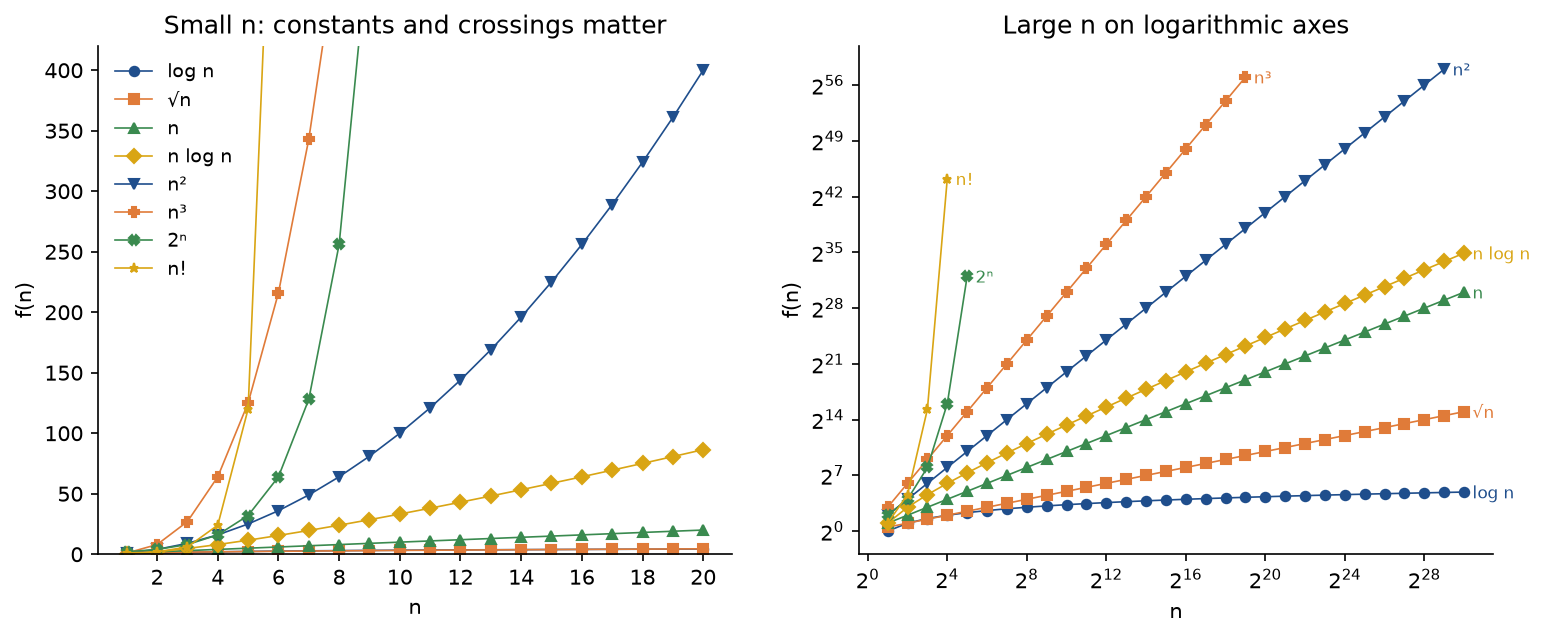
On the left, for small n, the curves cross and constants matter; on the right, on logarithmic axes, each polynomial is a straight line whose slope is its degree, and 2ⁿ and n! leave every polynomial behind within a few dozen values of n. The order from bottom to top is the order this page writes as 1 < log n < √n < n < n log n < n² < n³ < 2ⁿ < n!.

How it works

The random-access machine and what counts as a step

A cost model needs a machine. The random-access machine, or RAM, is an idealised computer with a processor that holds a few words in registers and a memory of numbered cells, each holding one word. One step is one primitive operation: an arithmetic or logical operator, a comparison, reading or writing one memory cell by its address, a jump, a call or a return. Every step costs the same, which is why this is called the unit-cost model.

The consequence that matters most is in the note on the left: a statement with a fixed shape costs a fixed number of steps, whatever the input. statement_cost in ram.py counts them by walking the statement's syntax tree. total = total + prices[k] * counts[k] reads two cells, applies two operators and stores one variable, 5 steps. found = low <= key and key < high makes two comparisons, one logical operator and one store, 4 steps. Whether the store counts, or whether an array read costs one step or two, changes these numbers, but every reasonable convention gives some constant, and the constant is what asymptotic notation is designed to ignore. Two-dimensional arrays show the same thing: cell (r, c) of a table with w columns stored row after row lives at r·w + c, so cells[r * width + c] = cells[(r - 1) * width + c] + 1 costs 8 steps, 6 of them arithmetic, while the list-of-lists version grid[r][c] = grid[r - 1][c] + 1 costs 6, with four reads of which two fetch a row. Both are constants.

The note on the right lists the traps. A loop is not one step, and neither is a single line that hides a loop: x in a_list compares x with each item in turn, sorted(a) makes about n log2 n comparisons, a[i:j] copies j − i references. The unit-cost model also assumes that every number fits in one machine word of w bits. Arithmetic on longer numbers costs more:

With 64-bit words, multiplying two 64-bit numbers is 1 word step, two 1024-bit numbers 256 and two 4096-bit numbers 4096, which is why an analysis that multiplies ever-growing integers, as computing large Fibonacci numbers or factorials does, must not charge one step per multiplication. The common rule is that numbers of O(log n) bits, enough to index the input, are free to treat as one word.

The package turns this model into a measuring tool. OperationCounter in counting.py is a small dataclass with one field per kind of operation, steps, comparisons, moves, stores, arithmetic, accesses, calls and hashes; every algorithm in the handbook takes an optional counter and adds to the fields it uses, and counter - before gives the cost of a single operation. Code we cannot instrument, such as the built-in max or sorted, is measured by handing it CountedKey objects, which count every comparison and hash made on them. Arbitrary Python functions are measured by count_lines in profiling.py, which adds one step for every line of Python executed, the closest a running program comes to the RAM's steps.

Counting loops exactly

The cost of a loop is the sum, over its iterations, of the cost of its body. Two rules follow, and confusing them is the most common error in loop analysis. Loops one after the other add: for i in range(n) followed by for j in range(n) runs 2n bodies. Loops nested inside each other multiply when their bounds are independent: for i in range(n): for j in range(n) runs n·n = n² bodies. An inner loop with a constant bound, such as for k in range(8), multiplies by that constant only, 8n bodies, still Θ(n).

When the inner bound depends on the outer index, the count becomes a sum. With for i in range(n): for j in range(i, n), the inner loop runs n times for i = 0, n − 1 times for i = 1, and once for i = n − 1:

A third dependent loop, for k in range(j, n), visits every triple i ≤ j ≤ k once:

Loops that change their variable by a factor are logarithmic. Halving m from n until it reaches 1 takes ⌊log2 n⌋ rounds, and doubling i from 1 while it stays below n takes ⌈log2 n⌉:

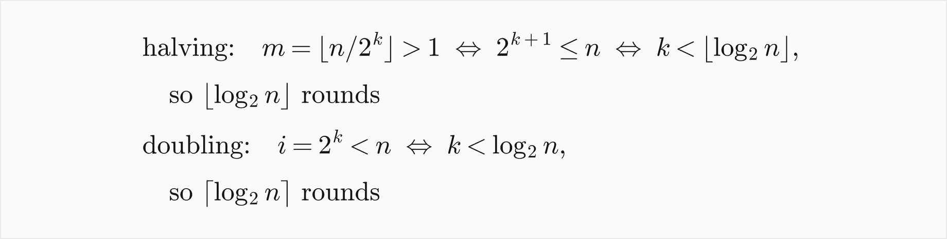
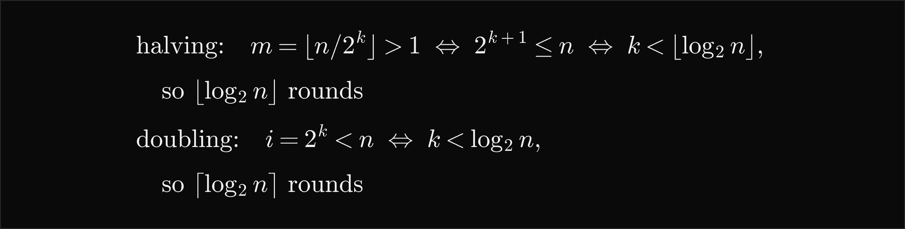
The floor and the ceiling are not decoration: for n = 37 the halving loop runs 5 times and the doubling loop 6 times, as the worked example traces. A doubling loop inside a linear one costs n(⌊log2 n⌋ + 1), Θ(n log n):

Some loops have a body whose cost varies from one iteration to the next, and then the nested shape misleads. In m = n; while m >= 1: for k in range(m): ...; m //= 2 the inner loop runs n, then about n/2, then n/4 times, a geometric series:

The two loops are nested, yet the total is Θ(n). The opposite shape, a cheap body with an occasional expensive one, behaves the same way. A loop that does one step per iteration plus i extra steps whenever i is a power of two, as a growing array that copies itself when it fills up does, costs

so each of its n iterations costs less than three steps on average, the idea behind Amortized analysis. A loop that stops when i² passes n runs ⌊√n⌋ times:

Finally, nested loops whose inner index is never reset cost the sum of their moves, not the product. A sliding window over items whose weights repeat 1, 1, 1, 3, kept within a budget of 4, adds the item at its right end each round and lets items go from its left end while the window is too heavy: left = 0; for right in range(n): add a[right]; while over budget: drop a[left]; left += 1. Some rounds let no item go and some let two go, but left only moves forward, so the inner loop runs at most n times over the whole run. Every item enters once and all but the w items of the final window leave once, so the count is exactly 2n − w, with w equal to 3 when n leaves remainder 3 on division by 4 and 2 otherwise, once n ≥ 4. Two-pointer scans such as the merge step of Merge sort are analysed the same way. All fifteen shapes live in loops.py, each paired with its closed form in shapes.py, and the tests compare the two for every n up to 300, or 40 for the triple loop.

Big O, Omega and Theta

Exact counts are useful but unwieldy; n(n + 1)(n + 2)/6 says more than anyone needs. Asymptotic notation keeps the growth and drops the rest, and it does so with explicit constants:

The constant c may scale g up as much as needed, and the inequality only has to hold from n0 on.

Ω is the mirror image: some multiple of g, scaled down if necessary, stays below f from n0 on.

O is an upper bound, Ω a lower bound and Θ both at once, each up to a constant factor and only from some n0 on. The constants are what make "asymptotic" precise: c absorbs the machine, the language and the cost convention, and n0 lets small inputs behave however they like. The equals sign is traditional but misleading. O(g) is a set of functions, and f(n) = O(g(n)) means f is a member of it; the statement cannot be read backwards, and n = O(n²) is true while n² = O(n) is false.

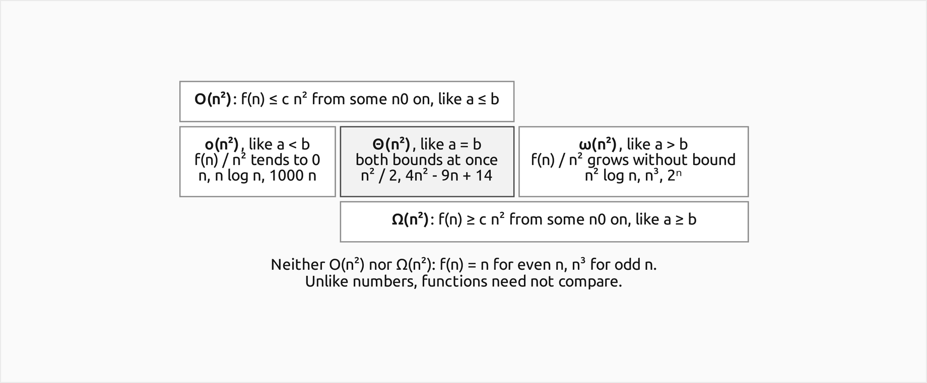
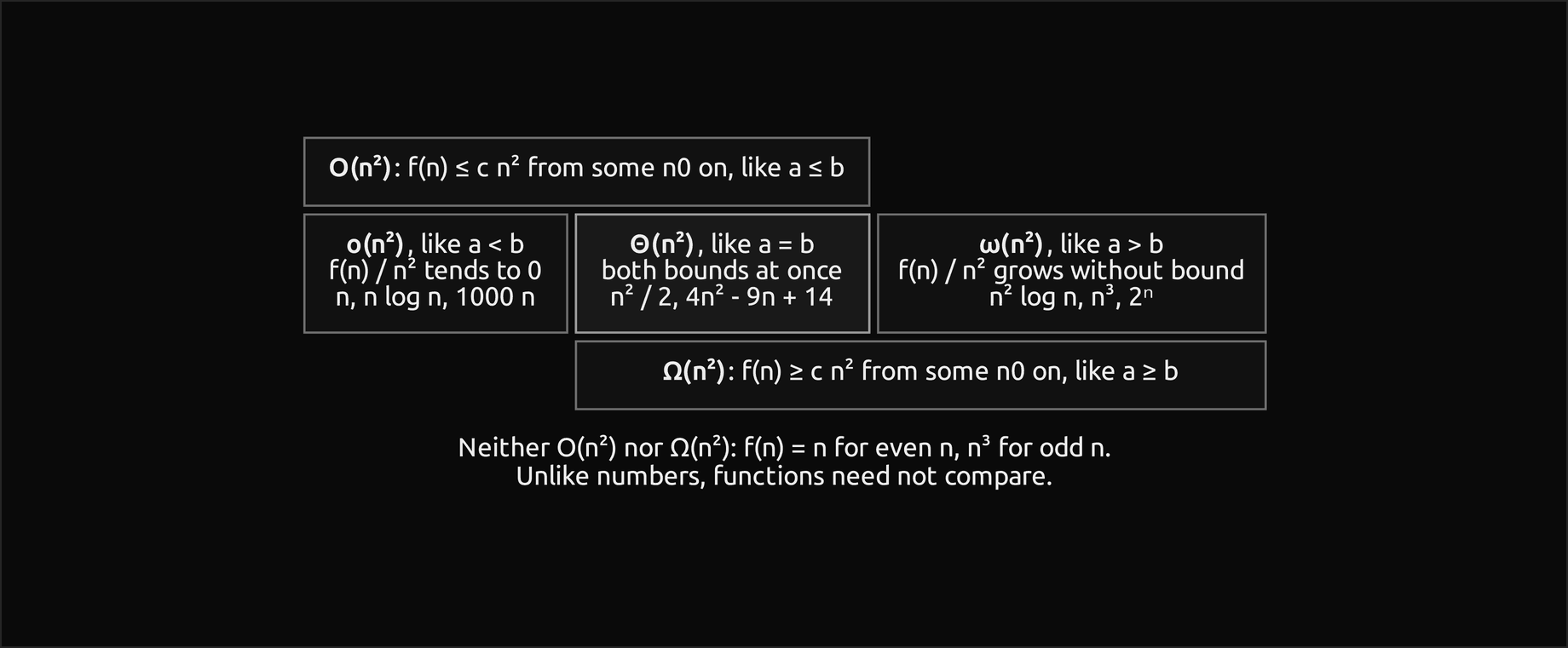
The diagram shows how the five relations fit together for g(n) = n². They behave like ≤, <, =, > and ≥ between numbers, with one difference, written under the cells: two functions need not be comparable at all, as the function equal to n for even n and n³ for odd n shows against n².

Two rules do most of the everyday work. Sums are dominated by their largest term and products multiply:

So a polynomial is Θ of its leading term, two sequential loops cost as much as the more expensive one, and nested loops cost the product. The base of a logarithm never matters inside O or Θ, because changing the base multiplies by a constant:

A loop that divides by 3 runs ⌊log3 n⌋ times, about 1.585 times fewer than a halving loop, which is a constant factor: both are Θ(log n). The base does matter in an exponent, where 2^(log2 n) = n but 4^(log2 n) = n².

Finding the constants c and n0

To prove a bound, exhibit c and n0 and show the inequality for every n ≥ n0. For a polynomial with a positive leading coefficient, algebra gives an upper witness at once: for n ≥ 1 every negative term is at most 0 and every positive term a·nᵏ is at most a·nᵈ, so c can be the sum of the positive coefficients and n0 = 1. On the function of the worked example, f(n) = 4n² − 9n + 14:

For a lower bound a subtracted term cannot simply be thrown away: removing −9n increases the expression, so the inequality would no longer follow. Positive lower terms can go, since they only make f larger; each negative term −b·nᵏ with k < d is at least −b·n^(d−1) for n ≥ 1; and a share of the leading term, half of it below, absorbs those negative terms once n is large enough:

upper_witness and lower_witness in notation.py apply these two recipes to any polynomial with integer coefficients, and upper_derivation and lower_derivation print the steps. The recipes are safe but loose. Many pairs (c, n0) work, and a larger c usually allows a smaller n0; the leading coefficient itself is the boundary. For the worked f, any c above 4 gives an upper bound and any c below 4 a lower bound, but c = 4 fails as a lower bound for every n ≥ 2, because 4n² − 9n + 14 < 4n² as soon as 9n > 14.

A search finds the smallest n0 for a chosen c. smallest_n0 checks the inequality from a limit downwards and returns one past the largest n where it fails. Walking down matters: the inequality 4n² − 9n + 14 ≥ 3n² holds at n = 1 and n = 2, fails for n = 3 to 6 and holds again from 7 on, because the difference is n² − 9n + 14 = (n − 2)(n − 7). The first n where a bound holds is therefore not a valid n0; the smallest valid one here is 7:

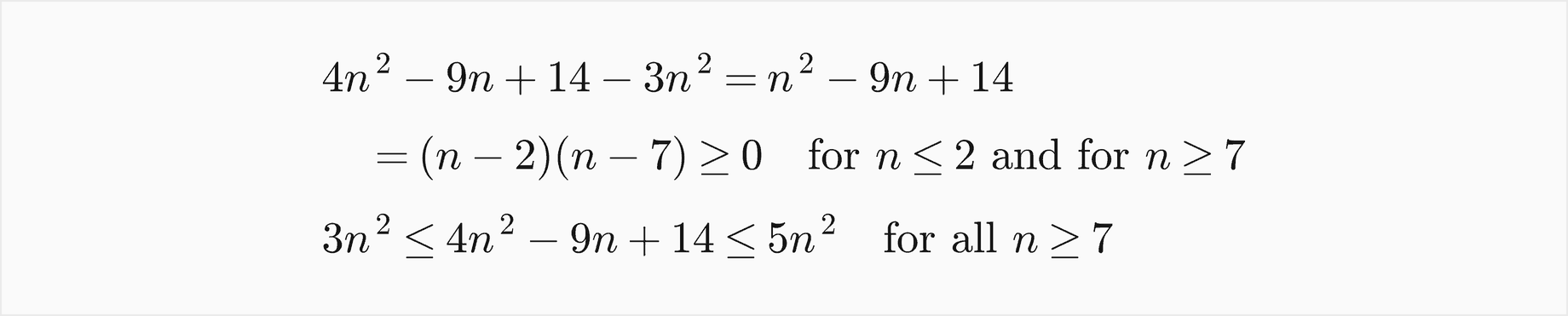
A search over a finite range is evidence, not proof: it cannot see beyond its limit. n² ≤ 1000n holds for every n up to 1000 and fails forever after, so a check up to 500 would "confirm" the false claim n² = O(n). Use the search to guess the constants and the algebra to prove them.

Little o, little omega and the limit test

The strict relations ask for more: the bound must hold for every constant, however small or large.

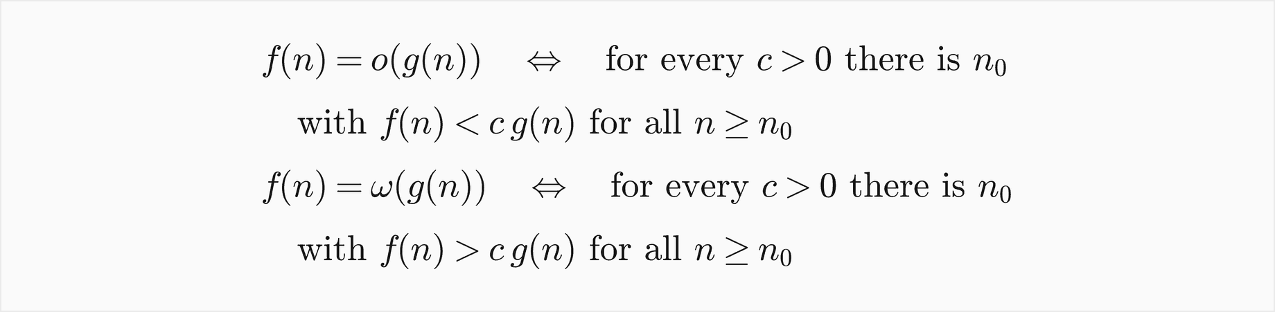
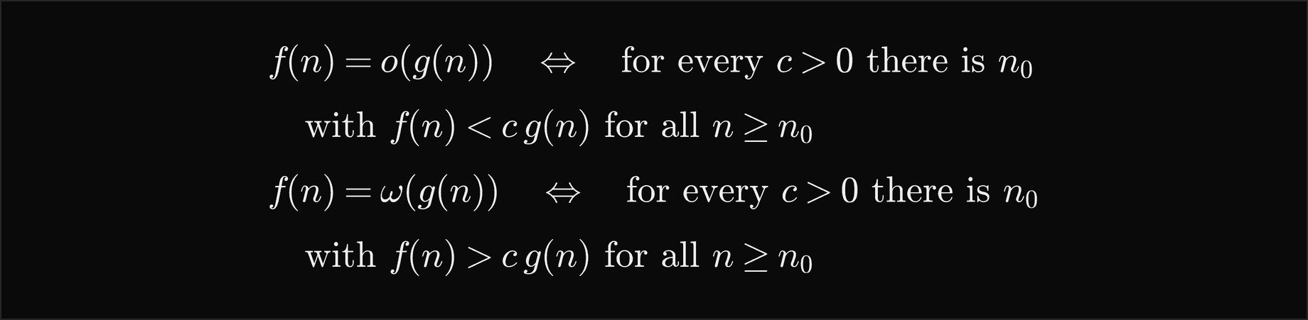
10n = o(n²): for c = 1, 0.1, 0.01 and 0.001 the thresholds are n0 = 11, 101, 1001 and 10001. Each smaller c needs a larger n0, but none fails. A function is never o of itself, and n² = O(n²) while n² ≠ o(n²). When the ratio f(n)/g(n) has a limit, the limit decides the relation:

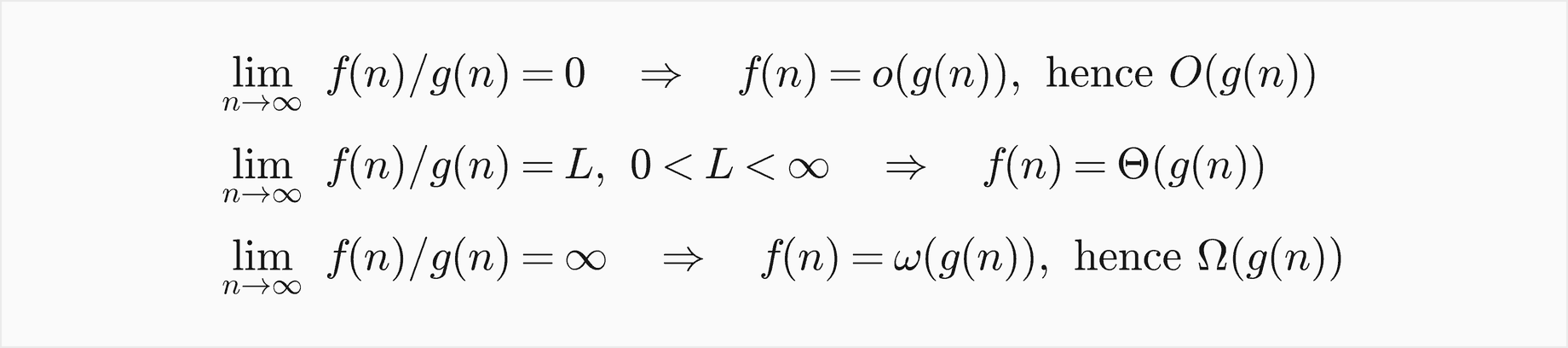
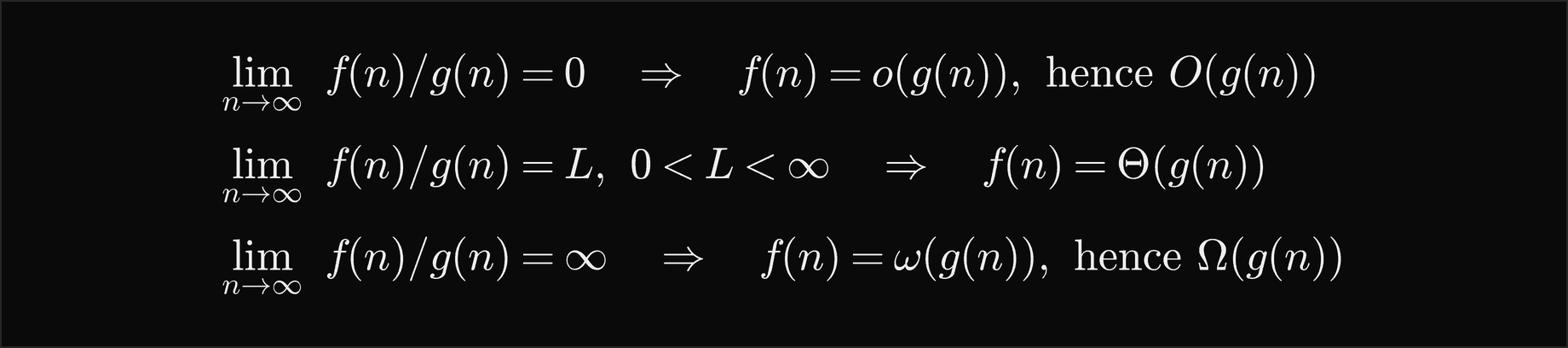
For polynomials with positive leading coefficients the limit is the ratio of the leading coefficients when the degrees agree, which polynomial_limit computes; the ratio (4n² − 9n + 14)/n² is 3.4922 at n = 16, 3.9651 at 256, 3.9978 at 4096 and 3.9999 at 65536, closing in on 4. The limit test is only a sufficient condition. The function equal to n for even n and 3n for odd n lies between n and 3n, so it is Θ(n), yet its ratio to n alternates 1, 3, 1, 3 and has no limit. A missing limit proves nothing; fall back to the definition.

Best, worst and average cases

An algorithm does not have one running time for each n; it has one for each input. Grouping the inputs by size gives three functions:

The worst case W(n) is a guarantee, the best case B(n) a curiosity and the average case A(n) a prediction that is only as good as the probability model behind it. O, Ω and Θ are statements about functions, and each of the three cases is a function, so each can be bounded on its own: insertion sort has W(n) = Θ(n²) and B(n) = Θ(n). "Insertion sort is O(n²)" is true because every case is at most quadratic; "insertion sort is O(n)" is false, because O must cover every input of size n, and a bound on the best case covers only one. O does not mean worst case, and Ω does not mean best case.

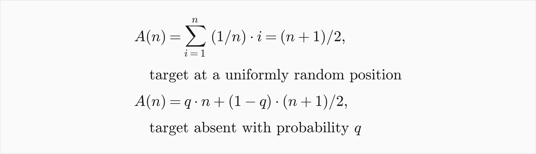
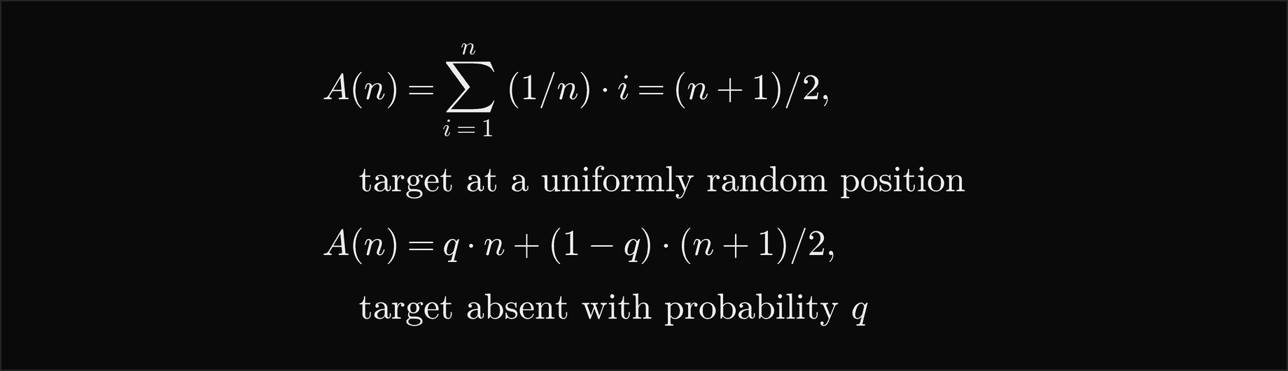
Three algorithms show the range. Linear search makes one comparison per probe: 1 in the best case, n in the worst, when the target is last or absent. If the target sits at a uniformly random position, the average is (n + 1)/2, and with an absent target mixed in at probability q the two cases mix:

Finding the maximum compares each later item once with the maximum so far: n − 1 comparisons for every input, so its three cases coincide. What varies is how often the maximum so far changes, which costs a store each time: never if the largest item comes first, n − 1 times if the items ascend. On a uniformly random order the i-th item beats all earlier ones with probability 1/i, since each of the first i items is equally likely to be their largest. Adding these chances with indicator variables gives a harmonic number, not half the items:

For n = 7 that is 223/140, about 1.5929 updates, not the (n − 1)/2 = 3 of the tempting argument "each later item is larger half of the time". The tool, linearity of expectation over indicator variables, is developed in Counting and probability for algorithms.

Insertion sort, traced in the worked example and treated fully in Elementary sorts, takes each item out of the array and shifts larger items of the sorted prefix one slot right until the item fits. Every shift removes one inversion, a pair of items in the wrong order, so the shifts equal the inversions: none on sorted input, n(n − 1)/2 on reversed input, and on average half of all pairs:

Each pass also makes one comparison that stops it, unless the item is the smallest so far and runs off the front of the array, which happens with probability 1/i for the i-th item:

cases.py checks all of these by brute force: it runs each algorithm on every ordering of n distinct keys for n up to 8, takes the minimum, maximum and exact mean as fractions, and the tests compare them with the closed forms.

Space and the call stack

Space is counted in cells the same way time is counted in steps. The usual measure is auxiliary space, the cells an algorithm needs beyond its input: reversing an array into a copy needs n new cells, reversing it in place by swapping from both ends needs one spare cell, Θ(1). A recursive function also uses the call stack, one frame per call that has started and not yet returned, and its stack space is the deepest chain of frames, not the number of calls:

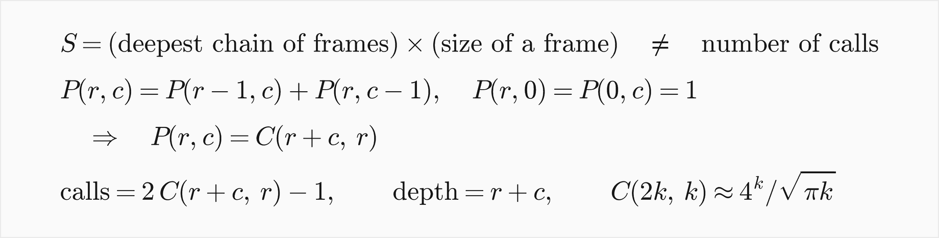
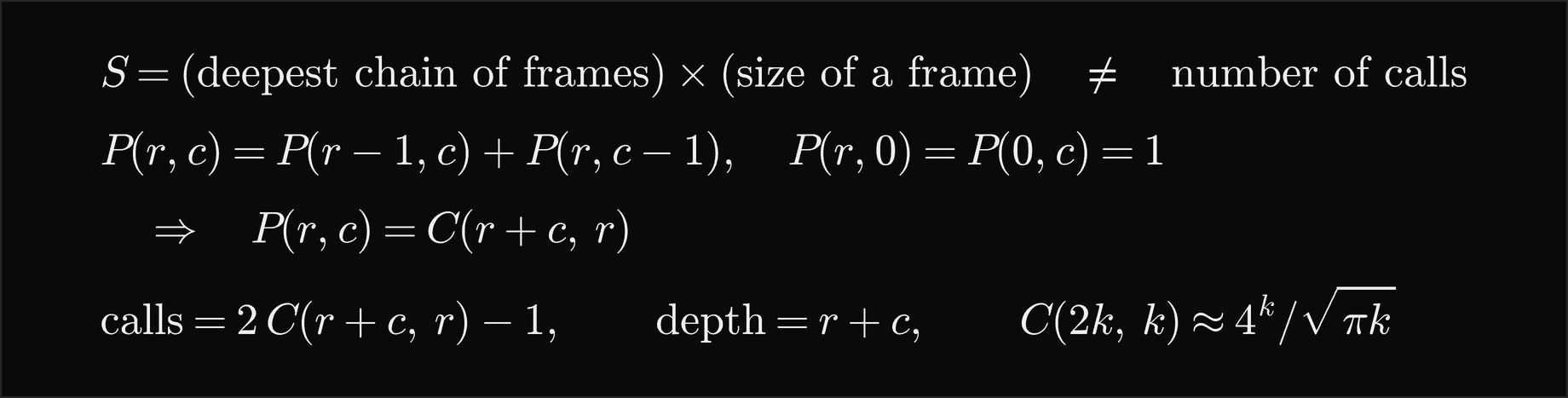
paths(r, c) counts the routes from the corner (r, c) of a grid to (0, 0) that move one unit down or one unit left at a time. It returns 1 on an edge, where r or c is 0, and otherwise adds paths(r - 1, c) and paths(r, c - 1). The answer is C(r + c, r), and since every call that does not return 1 at once makes two more, the calls number 2·C(r + c, r) − 1: 25739 for paths(8, 8), and about 2·4ᵏ/√(πk) on a k by k grid: exponential time. Yet the first of the two calls returns before the second starts, and each call lowers r + c by one, so the stack never holds more than r + c frames, 16 for paths(8, 8): linear space. The worked example draws the stack of paths(2, 2) call by call. A recursive binary search keeps one half of the range in each call, so it is ⌊log2 n⌋ + 2 frames deep at most, 21 frames when it looks past the last of 10⁶ keys, while a recursive sum of n values is n + 1 frames deep. That last kind is the dangerous one in Python, whose interpreter stops at about 1000 frames by default: summing 5000 numbers recursively raises RecursionError, while the loop that does the same needs one frame. The package never raises the limit; its recursive functions state their depth, and Recursion shows how to turn deep recursion into iteration.

Optimality and lower bounds

An upper bound describes one algorithm; a lower bound describes every algorithm for a problem in a stated model, and an algorithm whose worst case matches the lower bound is optimal in that model. Optimality is a claim about every algorithm the model allows, including those nobody has written yet, not about the fastest one found so far.

For the maximum in the comparison model, every item except the maximum must lose at least one comparison, otherwise it could still be the maximum, and each comparison has exactly one loser:

The scan makes exactly n − 1 comparisons, so it is optimal. The same argument can be played as a game against an adversary, which fool_maximum in lower_bounds.py does in code. It runs an algorithm, records the questions it asked and looks at them as a graph whose edges join the two items of each comparison. With fewer than n − 1 questions the graph has at least two separate groups. Adding the same large constant to every item of a group that does not contain the claimed maximum changes no answer, because no question compared items of different groups, so a deterministic algorithm asks the same questions and makes the same claim, which is now wrong.

The algorithm here is a knockout tournament that forgets the item without a partner whenever a round has an odd number of items. On seven values it asks only four questions and leaves three groups; raising the group of A[4] and A[5] makes 108 the true maximum while the tournament still answers A[1] = 64. On 2000 random inputs the adversary fooled it 1740 times and fooled a scan that skips the last item every time, while the correct scan and the correct tournament were never fooled.

For searching a sorted array with three-way comparisons, a decision tree lists every comparison an algorithm can make. Each node compares the target with one position; the outcome "equal" ends the search there, and "less" and "greater" lead to the left and right subtrees. A correct search must be able to end at each of the n positions, so its tree has at least n nodes, and a binary tree of height h has at most 2^h − 1:

Binary search meets the bound exactly: its decision tree is as balanced as a tree can be.

The tree has four levels for ten keys, and ⌈log2 11⌉ = 4. decision_tree builds this tree with the same middle rule as binary_search, and the tests check that its height equals the lower bound for every n up to 400. The same counting argument with n! leaves gives the Ω(n log n) bound for comparison sorting in The sorting lower bound and linear-time sorts.

Input size: values against bits

The size of an input is the number of symbols it takes to write down. For an array of n small numbers that is about n words, but for a single number N it is its length in bits, b = ⌊log2 N⌋ + 1, not N itself. An algorithm whose cost is polynomial in the value N can be exponential in the true size:

Testing a prime N by trial division tries every divisor up to √N: 14 divisions for the 8-bit prime 251, 254 for the 16-bit 65521, 4094 for the 24-bit 16777213 and 65534 for the 32-bit 4294967291. Every 8 more bits multiply the work by 16. Such algorithms are called pseudo-polynomial; the dynamic program for the 0/1 knapsack in Dynamic programming is another, polynomial in the capacity but not in its number of digits, and the distinction is the starting point of P and NP.

Cost

Loops counted against their closed forms

The example counting_steps.py runs every loop shape with a counter and compares the count with the closed form for every n below 65; all fifteen agree. For n = 1000 the counts are 1000 for a single loop, 2000 for two sequential loops, 8000 with a constant inner loop of 8, 1000000 for independent nested loops, 500500 for the dependent loop, 499500 for all pairs, 10000 for the doubling loop inside a linear one, 1994 for the shrinking loop, 2023 for the resizing loop and 1998 for the sliding window, while the halving loop stops after 9 rounds and the square-root loop after 31.

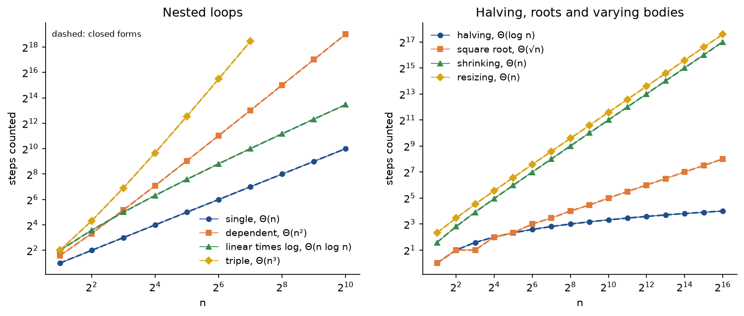
On logarithmic axes a count of Θ(nᵏ) is a straight line of slope k, so the picture reads off the class directly: the dependent loop has slope 2 although its count is half of n², the shrinking and resizing loops have slope 1 although both are nested, and the halving loop flattens. Every measured point sits on its dashed closed form.

Constants and thresholds

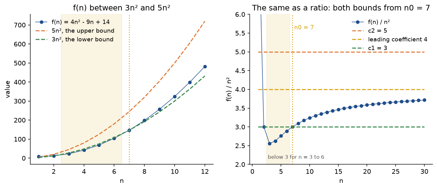
The right panel is the useful way to look at constants. The ratio f(n)/n² tends to the leading coefficient 4 from below, so any c1 under 4 eventually works and c1 = 4 never does, and the dip below 3 for n from 3 to 6 is why the smallest n0 for c1 = 3 is 7, not 1.

Constants also decide which algorithm wins at a given size. An algorithm costing 100 n log2 n steps is beaten by one costing n² until n² overtakes it, which happens from n = 997 on; 2ⁿ overtakes n⁴ from n = 17, n! overtakes 4ⁿ from n = 9, and n^1.5 overtakes 20n from n = 401. With a budget of 10⁹ steps, a few seconds of simple operations in C and minutes in pure Python, the largest input each class allows is about 10¹⁸ for √n, 10⁹ for n, about 3.96 × 10⁷ for n log2 n, 31622 for n², 1000 for n³, 29 for 2ⁿ and 12 for n!, while log n allows inputs larger than 2¹⁰⁰. That list explains more design decisions than any other number in this handbook: a quadratic algorithm is fine for a few thousand items and hopeless for a few million, and an exponential one is hopeless almost immediately.

Three cases of insertion sort

The example cases_and_lower_bounds.py first enumerates every ordering of n distinct keys for n up to 8 and confirms that the exact best, worst and average counts equal the closed forms, then measures larger sizes.

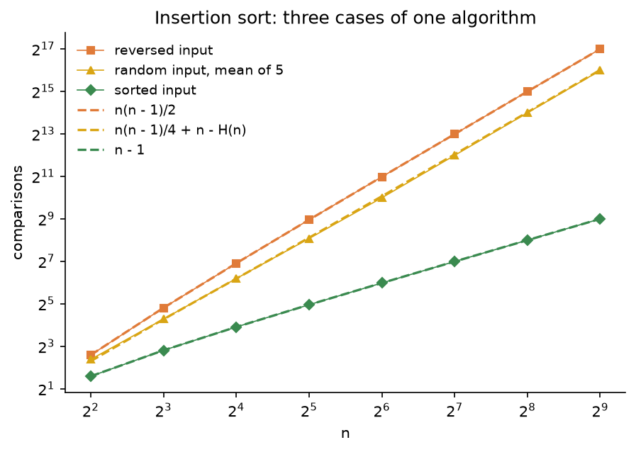
The worst and average cases are parallel lines of slope 2, a factor of two apart: on random input insertion sort does half the work of the worst case, still Θ(n²). The best case is a line of slope 1. At n = 512 the counts are 511 for sorted input, 130816 for reversed input and 64864.0 on average over five random permutations, against the predicted 65913.2; five samples land within about two percent.

The running maximum

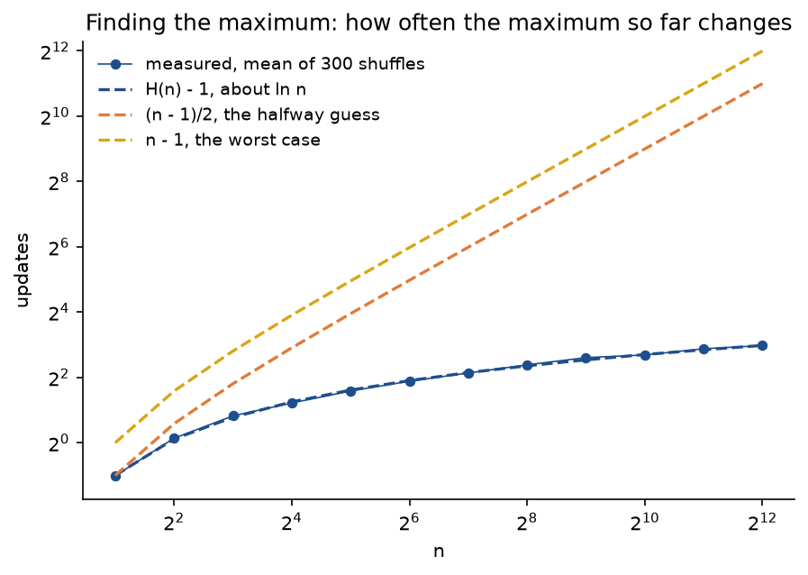
At n = 4096 the measured mean is 7.8700 updates against H(4096) − 1 = 7.8951, while the halfway guess predicts 2047.5. The comparisons stay at exactly n − 1 for every input; only the stores vary, and on random data they are a vanishing fraction of the work.

Time and space of recursion

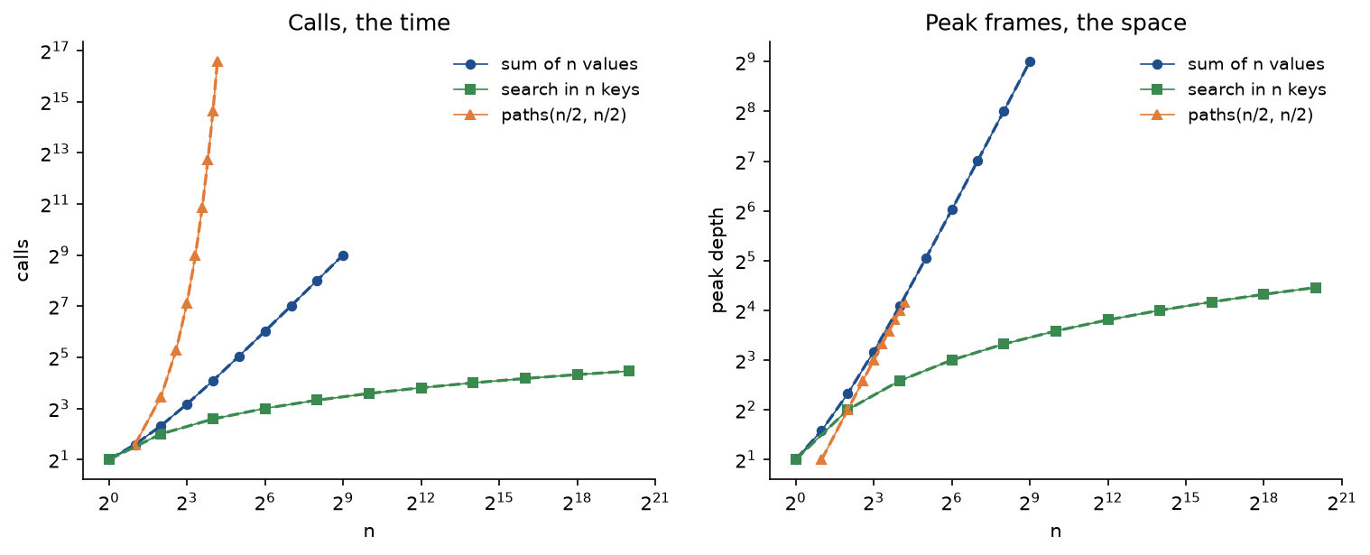
The left panel is time and the right panel is space. The path counter is exponential in time and linear in space: started at (9, 9) it makes 97239 calls with at most 18 frames, while the recursive sum over 512 values needs 513 frames for 513 calls.

Worked example

Every step below is printed by examples/worked_example.py and asserted by tests/test_worked_example.py.

Counting a loop nest exactly

The dependent loop for i in range(n): for j in range(i, n) with n = 5 runs its body for:

• i = 0: j from 0 to 4, 5 steps.
• i = 1: j from 1 to 4, 4 steps.
• i = 2: j from 2 to 4, 3 steps.
• i = 3: j from 3 to 4, 2 steps.
• i = 4: j = 4 only, 1 step.

The total is 15 = 5·6/2. The halving loop on n = 37 sets m to 18, 9, 4, 2 and 1 and stops: 5 rounds, and ⌊log2 37⌋ = 5 because 32 ≤ 37 < 64. The doubling loop runs its body with i = 1, 2, 4, 8, 16 and 32 and stops when i reaches 64: 6 rounds, and ⌈log2 37⌉ = 6.

Witnesses for a Θ bound

Show that f(n) = 4n² − 9n + 14 is Θ(n²). The values for n = 1 to 8 are 9, 12, 23, 42, 69, 104, 147 and 198, against 3n² = 3, 12, 27, 48, 75, 108, 147, 192 and 5n² = 5, 20, 45, 80, 125, 180, 245, 320.

• Upper bound by algebra: drop −9n and raise 14 to 14n², so f(n) ≤ 18n² for n ≥ 1: c = 18, n0 = 1.
• Upper bound by search with c = 5: f(1) = 9 > 5 fails, and from n = 2 on f(n) ≤ 5n², since 5n² − f(n) = n² + 9n − 14 is positive from n = 2: n0 = 2. With c = 4 the smallest n0 is also 2.
• Lower bound by algebra: drop 14 and absorb 9n with half of 4n²: f(n) ≥ 2n² once 4n − 9 ≥ 2n, that is n ≥ 4.5: c = 2, n0 = 5. A search with c = 2 finds that n0 = 1 already works, because 2n² − 9n + 14 has no real root.
• Lower bound by search with c = 3: the bound holds at n = 1 and 2, fails at n = 3, 4, 5 and 6 (23 < 27, 42 < 48, 69 < 75, 104 < 108) and holds from n = 7 on, where 147 = 147: n0 = 7.
• Lower bound with c = 4: f(n) ≥ 4n² needs 14 ≥ 9n, which fails for every n ≥ 2. No n0 exists.

So 3n² ≤ f(n) ≤ 5n² for all n ≥ 7, and f(n) = Θ(n²) with c1 = 3, c2 = 5 and n0 = 7.

The three cases of finding the maximum

The scan over 31, 12, 47, 26, 53, 8, 39 starts with 31 as the maximum so far:

• 12 against 31: not larger.
• 47 against 31: larger, the maximum so far becomes A[2] = 47.
• 26 against 47: not larger.
• 53 against 47: larger, the maximum so far becomes A[4] = 53.
• 8 against 53: not larger.
• 39 against 53: not larger.

That is 6 comparisons, n − 1 as always, and 2 updates. The best case for updates is 0, when the largest item comes first, and the worst is 6, when the items ascend. For the average, take all 24 orderings of four distinct keys: 6 of them need 0 updates, 11 need 1, 6 need 2 and 1 needs 3, so the mean is (0 + 11 + 12 + 3)/24 = 26/24 = 13/12, about 1.0833, which is H(4) − 1 = 1/2 + 1/3 + 1/4. For the seven items above the expected number is H(7) − 1 = 223/140, about 1.5929.

Insertion sort pass by pass

Insertion sort of 29, 14, 37, 8, 21, with the sorted prefix before the bar:

• Pass 1 takes 14: 14 < 29, shift 29 to A[1], place 14 at A[0]: [14, 29 | 37, 8, 21]. One comparison, one shift.
• Pass 2 takes 37: 37 ≥ 29, stop and place 37 at A[2]: [14, 29, 37 | 8, 21]. One comparison, no shift.
• Pass 3 takes 8: 8 < 37, 8 < 29 and 8 < 14, shifting all three, and place 8 at A[0]: [8, 14, 29, 37 | 21]. Three comparisons, three shifts; there is no stopping comparison because 8 ran off the front.
• Pass 4 takes 21: 21 < 37 and 21 < 29, shifting both, then 21 ≥ 14 stops: [8, 14, 21, 29, 37]. Three comparisons, two shifts.

The filled cell is the item placed in each pass and the outlined cells are those that received a shifted item; the gap after the sorted prefix plays the part of the bar in the trace. The sort makes 8 comparisons and 6 shifts, and the input has exactly 6 inversions: (29, 14), (29, 8), (29, 21), (14, 8), (37, 8) and (37, 21). For n = 5 the best case is 4 comparisons, the worst 10 and the average 463/60, about 7.7167, with 5 shifts on average, so this input is slightly worse than average.

Binary search and its decision tree

Searching 4, 9, 15, 22, 30, 38, 43, 51, 60, 72 for 43 follows the path of heavier edges in the decision tree above:

• Range A[0..9], probe A[4] = 30: 43 > 30, go right.
• Range A[5..9], probe A[7] = 51: 43 < 51, go left.
• Range A[5..6], probe A[5] = 38: 43 > 38, go right.
• Range A[6..6], probe A[6] = 43: found.

Searching for the absent 25 probes A[4] = 30 (go left), A[1] = 9, A[2] = 15 and A[3] = 22 (go right each time) and stops when the range A[4..3] is empty. Both searches take 4 probes, the height of the tree and the lower bound ⌈log2 11⌉ = 4.

The call stack of a recursion

paths(2, 2) calls paths(1, 2), which calls paths(0, 2) and returns 1 at once, then paths(1, 1), which calls paths(0, 1) and paths(1, 0). Back at the top, paths(2, 1) repeats the pattern: paths(1, 1) with its two edge calls, then paths(2, 0). The eleven calls start with 1, 2, 3, 3, 4, 4, 2, 3, 4, 4 and 3 frames on the stack, and the counter returns 6, the number of routes from (2, 2) to (0, 0).

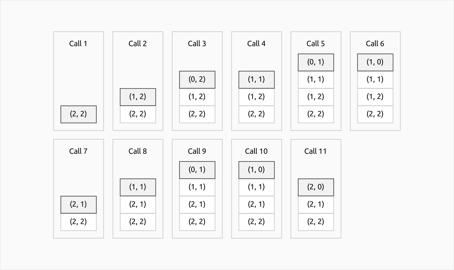
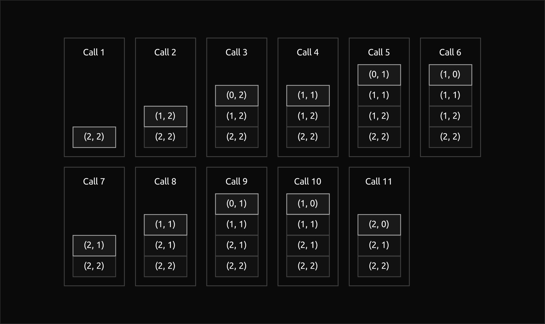
Eleven calls, 2·C(4, 2) − 1, but never more than four frames, r + c: the time is the number of snapshots and the space is the height of the tallest one.

Fooling a maximum algorithm

The broken tournament on 27, 64, 15, 42, 58, 33, 49 asks four questions: is A[0] < A[1]? yes; is A[2] < A[3]? yes; is A[4] < A[5]? no; and in the second round, with A[4] dropped, is A[1] < A[3]? no. It claims A[1] = 64 after 4 comparisons, below the lower bound of 6. The questions leave the groups {A[0], A[1], A[2], A[3]}, {A[4], A[5]} and {A[6]}. Adding 50, one more than the spread 64 − 15, to the second group gives 27, 64, 15, 42, 108, 83, 49: every answer stays the same, the tournament claims A[1] again, and the maximum is A[4] = 108. The figure in the section on lower bounds shows the four questions.

The code

The package asymptotic_analysis is plain Python, one idea per module. Importing it needs only the standard library; Matplotlib is imported by plotting.py alone.

• counting.py holds OperationCounter, with the fields steps, comparisons, moves, stores, arithmetic, accesses, calls and hashes, ensure_counter, and CountedKey, which counts the comparisons and hashes built-ins make.
• trace.py holds the Step record, record, describe, format_trace and format_array.
• ram.py holds statement_cost, which prices a Python statement in unit-cost steps, row-major addressing, word costs for long numbers and trial division as the pseudo-polynomial example.
• sums.py holds the exact closed forms: triangular and tetrahedral numbers, floors and ceilings of log2 computed from bit lengths, harmonic numbers as fractions, Σ⌊log2 k⌋ and Σ⌊n/2ᵏ⌋.
• loops.py holds fifteen counted loop shapes and shapes.py pairs each with its loop header, closed form and growth class.
• notation.py holds bound_holds, smallest_n0, theta_n0, little_o_thresholds, ratios, the Polynomial class and the algebraic witnesses with their printed derivations.
• growth.py holds the common growth functions, overtakes and largest_feasible for budgets.
• scans.py holds linear_search and find_maximum; insertion_sort.py holds insertion_sort and inversions; binary_search.py holds binary_search and its decision_tree.
• cases.py holds summarize, which takes the best, worst and exact mean cost over a set of inputs, and every closed form of the case analyses.
• lower_bounds.py holds the ComparisonOracle, the scan and tournament for the maximum, fool_maximum and the two lower bounds.
• space.py holds the SpaceMeter and the recursions and reversals it measures.
• containers.py measures list, deque, set and dict with wrapped keys and models the moves of a contiguous array; comparisons.py sets the built-ins max, in, bisect and sorted beside the package.
• profiling.py holds count_lines, which counts executed lines of Python with sys.settrace, and fit_growth, which fits a growth class to counts.
• invariants.py holds the checks the tests run: witness_violation, running_maximum_violation, sorted_prefix_violation, check_insertion_trace and decision_tree_violation.
• workloads.py holds the worked example's inputs and seeded random inputs; pitfalls.py holds the wrong analyses and misleading functions of the Pitfalls section; drawing.py writes the generated diagrams of arrays and call stacks as grids of captioned frames, tree_drawing.py writes the decision tree and the comparison graph, grid.py holds the shared style and the grid of frames, layout.py computes the tidy tree layout that pins every node so a left child stays on the left, and plotting.py draws the figures.

Counting never changes what the code does. The scan for the maximum adds to the counter where the RAM would spend a step:

for index in range(1, len(values)):
    counter.comparisons += 1
    larger = values[index] > values[best]
    if larger:
        best = index
        counter.stores += 1

The examples run in a few seconds each from the repository root:

• examples/worked_example.py prints every step of the worked example and writes the four generated diagram sources.
• examples/counting_steps.py prices statements, counts every loop shape against its closed form, measures the calls and frames of three recursions, and shows word costs and trial division.
• examples/notation_and_growth.py finds witnesses by algebra and by search, prints little-o thresholds, limit ratios, crossovers and the budget list, and draws the growth of the common functions.
• examples/cases_and_lower_bounds.py enumerates every input of small sizes, measures larger ones, and runs the adversary and the decision-tree check.
• examples/compare_with_builtins.py checks the package against max, in, bisect and sorted, counts the containers and prints rough timings.
• examples/common_mistakes.py runs every wrong analysis from pitfalls.py next to the correct count.
• examples/practice.py prints fresh exercises with their solutions; --seed gives a new set.

python foundations/asymptotic-analysis/examples/worked_example.py
python foundations/asymptotic-analysis/examples/counting_steps.py
python foundations/asymptotic-analysis/examples/notation_and_growth.py
python foundations/asymptotic-analysis/examples/cases_and_lower_bounds.py
python foundations/asymptotic-analysis/examples/compare_with_builtins.py
python foundations/asymptotic-analysis/examples/common_mistakes.py
python foundations/asymptotic-analysis/examples/practice.py --seed 7

The sample project, project/profile_growth.py with its helpers project/subjects.py and project/harness.py, is a growth profiler. It takes twelve ordinary Python functions written without any counting code: a closed-form sum, binary search, modular exponentiation by squaring, primality by trial division, three ways to detect a duplicate (with a set, by sorting, and by comparing all pairs), merge sort, removing duplicates with a list, insertion sort, matrix multiplication and the naive recursive Fibonacci function. For each one it builds inputs of growing size, runs the function under count_lines with the list items wrapped in CountedKey, so that it counts both the lines of Python executed and the comparisons and hashes made on the keys, including those inside built-ins, and fits the growth class of both counts with fit_growth. Sizes double until a function reaches a budget of counted operations; when one doubling multiplies the count by more than 16, faster than n⁴, the harness switches to small steps, which is how it gathers enough points for exponential growth. Options --budget, --subjects, --seed, --list and --figures change the run, and the default run takes about 5 seconds.

python foundations/asymptotic-analysis/project/profile_growth.py
python foundations/asymptotic-analysis/project/profile_growth.py --subjects fibonacci,merge_sort --budget 2000000

The fit works on the larger half of the sizes, where lower-order terms have faded. Exponential growth makes the logarithm of the count a straight line in n, polynomial growth a straight line in log n; if the first fits better and climbs, the result is exponential with the fitted base, and otherwise the class g whose ratio count/g(n) has the flattest slope on logarithmic axes wins. In the default run all 18 fitted classes, 12 for lines and 6 for key operations, agree with the analysis, including the base 1.618 of the Fibonacci recursion, the golden ratio. Two functions are flagged for hiding their work inside one line: has_duplicate_sorted executes 65537 lines at n = 32768 but makes 481632 comparisons and hashes inside sorted, Θ(n log n) behind Θ(n) lines, and dedupe_with_list executes 3075 lines at n = 1024 but makes 523776 comparisons inside not in, Θ(n²) behind Θ(n) lines.

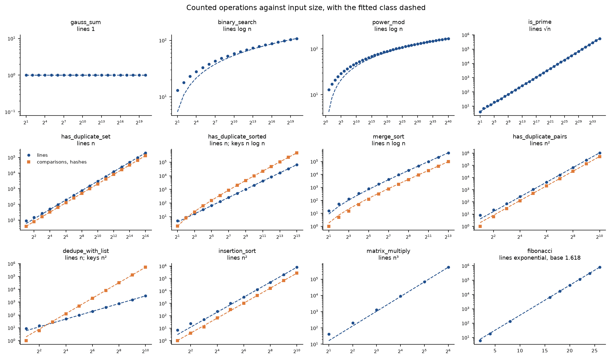
Each panel shows the lines in blue and the key operations in orange with their fitted classes dashed. The two flagged functions are the panels where the orange points climb more steeply than the blue ones: the lines alone would have called both linear.

The notebook asymptotic_analysis.ipynb follows this page: the RAM and statement costs, the loop shapes, witnesses and limits, the three algorithms' cases, space, lower bounds, the built-ins and a short run of the profiler. The tests in tests check the worked example value by value, every loop against its closed form, every case analysis by enumeration, the invariants, the agreement with the built-ins and the profiler's fits, and run in a few seconds:

python -m pytest foundations/asymptotic-analysis

All data are synthetic, generated from seeds by workloads.py and project/subjects.py, so nothing is downloaded and no licence is involved.

In practice

Python's built-ins against the package

The built-ins do the same work as the package, measured the same way. max over 1000 keys makes 999 comparisons, exactly like find_maximum. The in operator on a list makes the same comparisons as linear_search, one per item until it finds the target. bisect.bisect_left returns the same positions as binary_search but never stops early: it halves the range until it is empty, ⌊log2 n⌋ or ⌊log2 n⌋ + 1 two-way comparisons on every input, 9 to 11 including a final equality test on 1000 keys, where the three-way binary_search took 5 to 10 probes. sorted agrees with insertion_sort and needs only 8638 comparisons for 1000 random keys against 258998, but on already sorted input both make 999, n − 1, because Python's Timsort first looks for runs that are already in order.

from asymptotic_analysis import builtin_maximum, find_maximum, OperationCounter

values = [31, 12, 47, 26, 53, 8, 39]
counter = OperationCounter()
best = find_maximum(values, counter)
assert builtin_maximum(values) == (values[best], counter.comparisons) == (53, 6)

In wall-clock time the built-ins are much faster, which is the gap between C and interpreted Python and not a difference in growth: find_maximum was 20 to 35 times slower than max on 100000 keys over several runs, and binary_search about 40 times slower than bisect. These ratios vary from machine to machine and run to run; the counts do not.

What Python's containers cost

The costs below are those of CPython's implementation, average case first:

• list: reading or writing at an index, len, append and pop() from the end are O(1), with append amortized over the occasional resize. x in a, a.index(x), a.remove(x) and a.count(x) are O(n). a.insert(i, x) and a.pop(i) move every item after position i, O(n − i), so O(n) at the front. Slicing and copying are O(k) for k items, and sort is O(n log n), with n − 1 comparisons on sorted input.
• collections.deque: append, appendleft, pop and popleft are O(1) at both ends, because the deque is a linked list of blocks; indexing in the middle and x in d are O(n).
• set and dict: membership, lookup, insertion and deletion are O(1) on average, one hash and usually one comparison; the worst case is O(n) per operation when many keys share a hash.

The counts confirm each line. Looking up the last of n keys costs n comparisons in a list or a deque and one hash and one comparison in a set or dict, for n from 10 to 10000. A dict of 1000 keys with good hashes is built with 1000 hashes and no comparison, but when every key has the same hash it takes 499500 comparisons, n(n − 1)/2, the quadratic worst case that hash flooding attacks exploit, covered in Hashing in practice. Inserting 1000 items at the front of a contiguous array moves 499500 items, while appending them moves none; the model ShiftingArray counts those moves, which list.insert makes in C where no key can see them.

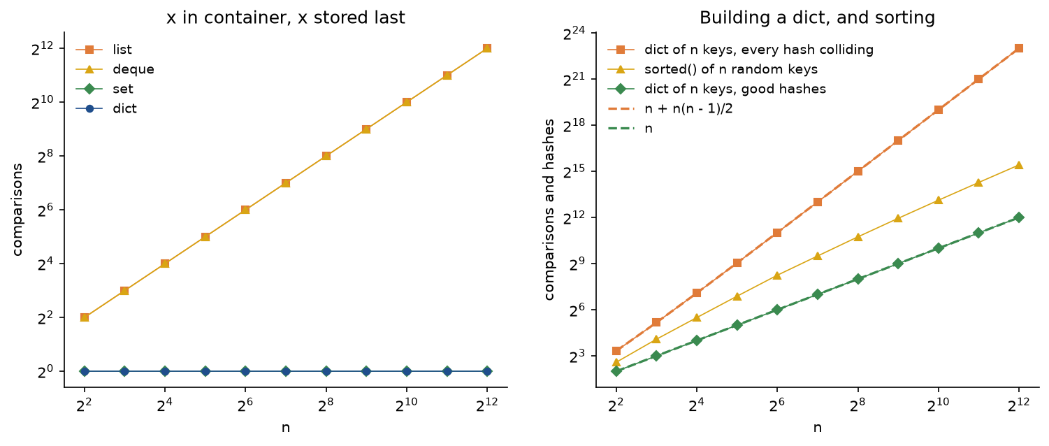
The timings tell the same story with C's constants: 30000 insertions at the front took about 130 times longer with list.insert(0, x) than with deque.appendleft, and 2000 membership tests in 10000 keys took on the order of a thousand times longer in a list than in a set. When to use which:

• Use a list for indexing and for appending and popping at the end; never use insert(0, x) or pop(0) in a loop on a long list.
• Use a deque for a queue or anything that adds or removes at both ends, see Queues and deques.
• Use a set or dict for membership and lookup by key, see Hash tables, and keep a list beside it when order matters.
• Use sorted or list.sort rather than any sort written in Python, and bisect on a sorted list for repeated searches.
• Read every line that calls a built-in as a loop of its own when analysing code: if x not in seen inside a loop is a nested loop when seen is a list.

Measuring in real projects

Counts explain growth; timings decide whether a program is fast enough. Python's timeit module times small snippets with repetition, cProfile reports where a program spends its time call by call, and sys.settrace, which count_lines uses, or sys.monitoring since Python 3.12, can count lines and calls when a deterministic measure is wanted. Honest timing takes the best of several runs, keeps inputs identical across the methods compared, and checks growth by doubling the input rather than trusting one size. C++'s standard library states the complexity of every container operation as part of its specification, Java's documentation does the same for its collections, and both, like Python's, give amortized or average costs where the worst case differs, which is the distinction this page draws between the three cases. The recurrences that arise from recursive algorithms are solved in Recurrences and the master theorem.

Pitfalls

• Adding the costs of nested loops or multiplying those of sequential ones. Nested loops with independent bounds multiply, n·n = 1000000 for n = 1000, while two loops one after the other add, 2000. examples/common_mistakes.py prints both mistakes next to the counts, and every following one as well.
• Calling a nested shape quadratic without counting. An inner index that is never reset, a halving inner bound or an occasional expensive body all give linear totals in nested loops: the sliding window makes 1998 steps for n = 1000, not 1000000.
• Taking n0 to be the first n where a bound holds. 4n² − 9n + 14 ≥ 3n² holds at n = 1, fails for n = 3 to 6 and holds again from 7. Search from the top down, or factor the difference, as (n − 2)(n − 7) shows here.
• Believing a finite check. n² ≤ 1000n holds for every n up to 1000 and is still false asymptotically. A search suggests constants; only algebra proves them.
• Dropping a negative term in a lower bound. Dropping −9n makes 4n² − 9n + 14 look at least 4n², which fails from n = 2. Absorb negative terms with a share of the leading term instead, so c must be below the leading coefficient.
• Confusing O with the worst case and Ω with the best case. O, Ω and Θ bound functions; the worst, best and average costs are three different functions, each with its own bounds. Insertion sort is not O(n), even though it makes only n − 1 comparisons on sorted input; reversed input of 1000 keys takes 499500.
• Averaging with the wrong model. The running maximum does not change on half of the later items; it changes H(n) − 1 times on average, 6.4855 for n = 1000 against the guess 499.5. State the input distribution, and prefer indicator variables to intuition.
• Treating one line as one step. item not in seen on a list, sorted, sum, slicing and string concatenation in a loop all hide loops. Removing duplicates from 1600 distinct items with a list executes 4803 lines but makes 1279200 comparisons.
• Worrying about the base of a logarithm, or forgetting it in an exponent. log2 n and log3 n differ by the constant factor log2 3, about 1.585, so Θ(log n) needs no base; but 2^(log2 n) = n while 4^(log2 n) = n².
• Reading a missing limit as a missing bound. The function equal to n for even n and 3n for odd n has no limit against n and is still Θ(n); the limit test is sufficient, not necessary.
• Counting calls as space. The path counter started at (9, 9) makes 97239 calls but never uses more than 18 frames; space is the deepest chain of frames. In Python, depth is the scarce resource: about 1000 frames by default.
• Measuring a number's size by its value. Trial division is polynomial in N but exponential in its b bits: 31621 divisions for the 30-bit prime 1000000007, about 32 times more for every 10 more bits.
• Comparing algorithms by asymptotic class alone at small sizes. 100 n log2 n is larger than n² until n = 997; constants decide below the crossover, which is why library sorts switch to insertion sort for short runs.

Further reading

• D. E. Knuth, The Art of Computer Programming, volume 1, Fundamental Algorithms, third edition, sections 1.2 and 1.3, Addison-Wesley, 1997. Sums, harmonic numbers, the analysis of the running maximum and the use of O.
• D. E. Knuth, "Big Omicron and big Omega and big Theta", ACM SIGACT News 8(2), 18-24, 1976. The paper that fixed the meaning of Ω and Θ used today.
• T. H. Cormen, C. E. Leiserson, R. L. Rivest and C. Stein, Introduction to Algorithms, fourth edition, chapters 2 and 3 and appendix C, MIT Press, 2022. The RAM model, insertion sort's cases and asymptotic notation.
• R. Sedgewick and P. Flajolet, An Introduction to the Analysis of Algorithms, second edition, Addison-Wesley, 2013. Exact average-case analysis, including left-to-right maxima and inversions.
• R. L. Graham, D. E. Knuth and O. Patashnik, Concrete Mathematics, second edition, chapters 2, 6 and 9, Addison-Wesley, 1994. Sums, harmonic numbers and asymptotics in depth.
• S. Baase and A. Van Gelder, Computer Algorithms: Introduction to Design and Analysis, third edition, chapter 1, Addison-Wesley, 2000. Optimality, the lower bound for the maximum and the decision-tree bound for search.
• J. Erickson, Algorithms, 2019, freely available at jeffe.cs.illinois.edu/teaching/algorithms. Clear treatments of recursion, the cost of recursive calls and lower bounds.
• E. Lehman, F. T. Leighton and A. R. Meyer, Mathematics for Computer Science, 2017, freely available from MIT OpenCourseWare. Asymptotic notation, sums and probability for algorithms.
• The Python wiki page TimeComplexity and the documentation of the collections, bisect, timeit and sys modules.