Hash tables

A dictionary stores values under keys and answers one question over and over: what is stored under this key? Search trees answer it in O(log n) comparisons by keeping the keys in order. A hash table gives up the order and answers in a constant expected number of steps, whatever the number of keys, by computing where a key belongs instead of searching for it. Python's dict and set, the symbol tables of compilers, database hash joins, caches and almost every deduplication or counting job rest on that trick. This page defines the dictionary abstract data type, builds hash functions and measures how evenly they spread real and synthetic keys, implements separate chaining and open addressing with linear probing, quadratic probing and double hashing, deletes with tombstones, grows the table as it fills, derives the expected number of probes for every strategy (including Knuth's formulas for linear probing) and checks every formula against counted probes, and shows primary and secondary clustering in pictures and numbers. Afterwards you will be able to fill a table by hand with any of the strategies, say which conditions make quadratic probing and double hashing safe, predict the cost of a search from the load factor, and choose between dict, set and a table of your own. It builds on Linked lists, Arrays and dynamic arrays and the expectations of Counting and probability for algorithms; Hashing in practice continues with Python's own dict, universal hashing and hash flooding.

The tables need only the standard library; to run the plots, the notebook and the sample project install the base group, and the project downloads two public-domain texts on its first run.

Intuition

Picture a cloakroom with thirteen numbered hooks and no list of whose coat hangs where. The attendant turns each guest's name into a hook number with a fixed rule and hangs the coat there; to give it back, they apply the same rule and walk straight to the hook. Nobody searches. The trouble starts when two names give the same number. The attendant can hang both coats on one hook, one behind the other, and check each when asked; or hang the second coat on the next free hook and remember that a coat may sit a little further along than its own number says. As long as there are more hooks than coats and the rule scatters the names well, almost every coat is found at the first or second hook the attendant tries, and that stays true whether the cloakroom holds thirteen coats or thirteen thousand, as long as the number of hooks grows with them.

That is a hash table. The rule is the hash function, two names that give the same number are a collision, hanging several coats on one hook is separate chaining, and taking the next free hook is open addressing. Everything else on this page is about making the rule scatter well, keeping the cloakroom from filling up, and knowing exactly how many hooks a search inspects.

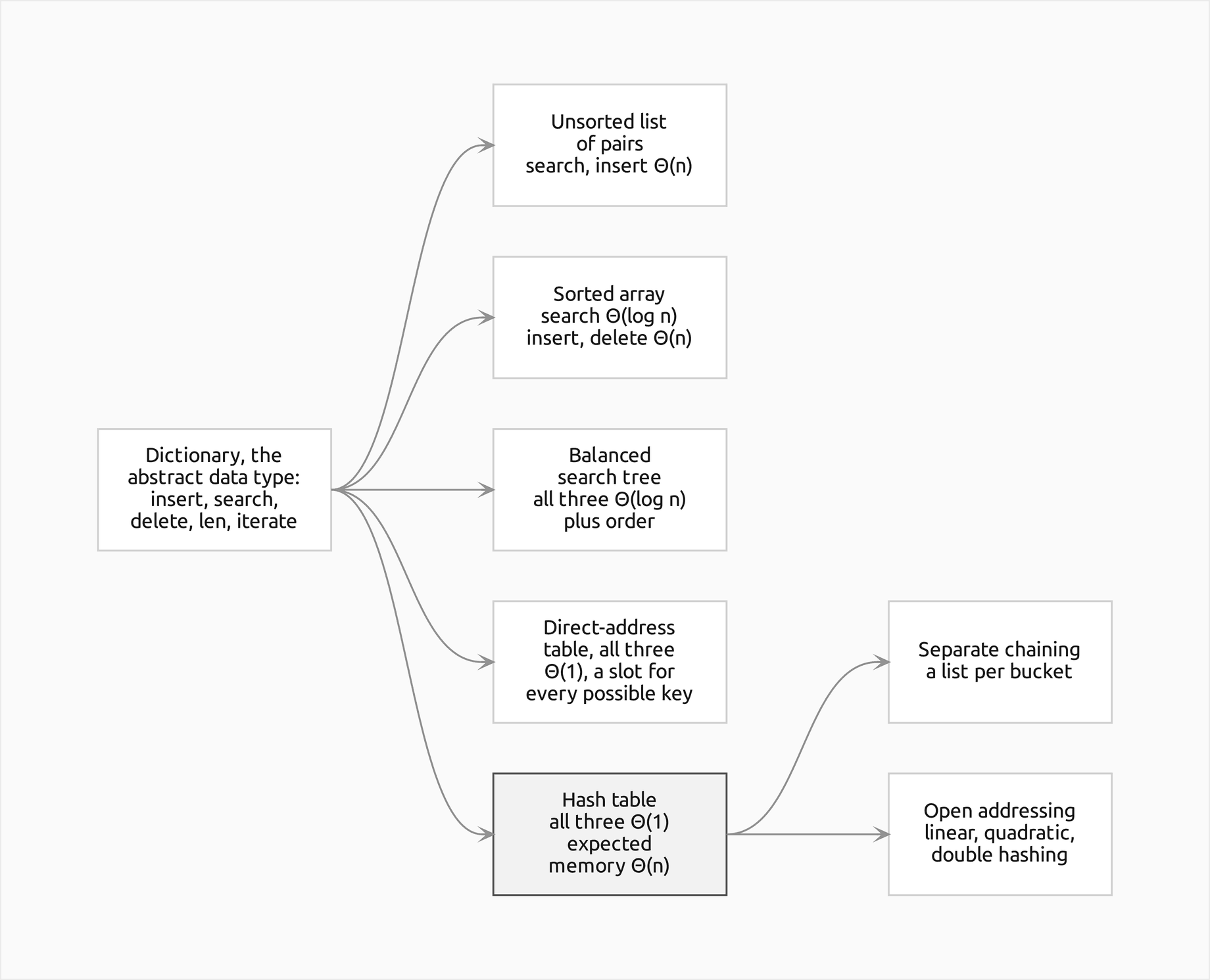
The diagram shows the abstract data type on the left and five ways to implement it. Only the hash table, the outlined box, makes all three operations constant on average while using memory in proportion to the number of keys stored; its two families of collision resolution sit to its right. Together they serve sets and counting, caches and memoization, symbol tables, indexes, joins and deduplication.

How it works

The dictionary abstract data type

A dictionary, also called a map, an associative array or a symbol table, holds pairs of a key and a value, with every key at most once. Its operations are:

• insert(key, value) stores the pair, replacing the value if the key is already present.
• search(key) returns the value stored under the key, or reports that the key is absent.
• delete(key) removes the key and its value.
• len() counts the keys, and iteration visits each key once.

Nothing is promised about the order in which keys come out, and there is no "next larger key": a dictionary only tests keys for equality. A set is a dictionary without values. In Python the contract is the MutableMapping interface, and every table in the package implements it, so table[key] = value, table[key], del table[key], key in table, len(table) and for key in table work as they do on a dict.

The implementations in the diagram trade differently. An unsorted list of pairs scans for every key, Θ(n). A sorted array finds a key by binary search in Θ(log n) comparisons but shifts Θ(n) elements to insert or delete one. A balanced search tree, such as an AVL tree, a red-black tree or a B-tree, does all three in Θ(log n) and also keeps the keys in order. The two remaining boxes are the subject of this page.

From direct addressing to hashing

When the keys are small integers, say from a universe of U possible values 0 to U − 1, the fastest dictionary of all is an array of U slots with the value of key k in slot k. That is a direct-address table: every operation is one array access. It fails as soon as the universe is large. Keys that are 64-bit integers, strings or tuples come from a universe far too large for an array, while the number n of keys actually stored is modest.

A hash table keeps the array but makes it only m slots long, with m proportional to n, and maps each key to a slot with a hash function h whose values lie between 0 and m − 1. The load factor says how full the table is:

Since the universe is larger than m, the pigeonhole principle guarantees that some keys share a slot, and much sooner than intuition suggests. Each of the n(n − 1)/2 pairs of keys collides with probability 1/m when keys land at random, so collisions start once n is around the square root of m:

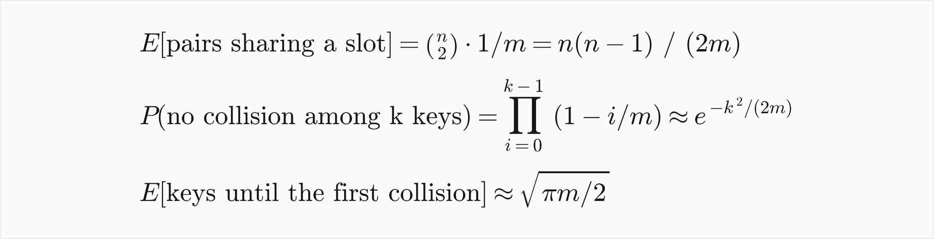
This is the birthday problem: with 365 slots the first collision is expected after about 24 keys. The example hash_function_quality.py throws keys at random into tables of 365, 1021 and 8191 slots 2000 times each; the first collision came after 24.79, 40.13 and 115.83 keys on average, against exact expectations of 24.62, 40.72 and 114.10. Collisions are therefore not an accident to be avoided but a normal event to be handled, and the two families of hash tables differ in how they handle it.

Hash functions

A hash function is best thought of in two stages. A hash code turns any key into a large integer, and a compression function turns that integer into a slot number from 0 to m − 1. The package's hash_code returns integers as they are, folds strings and tuples into an integer below the prime 2^61 − 1, and the tables then compress with the division method:

The division method is as fast as hashing gets, but it only uses the remainder of the key, so the choice of m matters. If m is a power of two, k mod m is just the lowest bits of k, and keys that agree in their low bits collide: multiples of 32, such as aligned addresses or identifiers handed out in steps, use only m/32 of the slots. A prime m that is not close to a power of two uses every part of the key, and an arithmetic progression of keys whose step shares no factor with m cycles through all m slots before repeating.

The multiplication method multiplies the key by a constant A between 0 and 1, keeps the fractional part and scales it to the table:

The fractional parts of k·A for consecutive k are spread almost evenly over the unit interval, best of all for Knuth's choice of A, the golden ratio's fractional part, so the method works for any m, including powers of two. The second line is how to compute it: with a w-bit integer s standing for A, the product k·s modulo 2^w is the fraction written as a w-bit number, and multiplying by m and keeping the bits above position w takes the floor. multiplication_hash does exactly that. The same formula in floating point quietly breaks for large keys, because a double holds 53 bits and the fractional part of k·A is lost once k·A passes 2^53: a thousand keys near 10^17 all landed in one slot of 1024 in floating point and in 930 different slots in integer arithmetic.

A string is a sequence of character codes, and a good string hash must let every character and its position change the result. The polynomial hash reads the string as the digits of a number in base B, computed by Horner's rule with a reduction after every step:

The package uses B = 31 and M = 2^61 − 1, a prime, and then reduces modulo m. The two weak alternatives show why both the weights and the base matter. Summing the character codes ignores positions, so all anagrams collide, and short words all fall into a narrow band of sums. A polynomial with base 32 reduced modulo 1024 keeps only the last two characters, because 32² is a multiple of 1024.

What makes a hash function good is now easy to list. It must be deterministic and agree with equality: equal keys must get equal codes, or a table cannot find what it stored. It must be cheap compared with the operation it serves. It must depend on every part of the key. And it must spread the keys that occur in practice as if they were thrown at random, which is the assumption every cost formula below is built on:

Under that assumption the number of keys in one bucket is binomial, and close to a Poisson distribution with mean α:

A single number measures how far a real function is from that ideal. With L_j keys in bucket j, the chi-squared statistic adds up the squared deviations from the mean; for random hashing its expectation is exactly m − 1, so the ratio χ²/(m − 1) is near 1 for a function that behaves randomly and far above 1 for one that clumps:

The example hash_function_quality.py measures four functions.

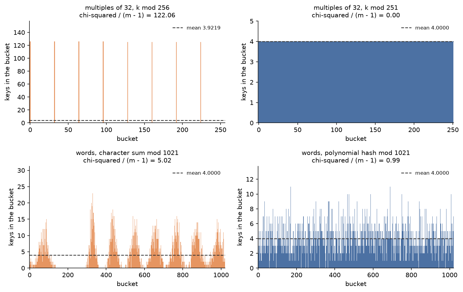
The power of two wastes 248 of its 256 buckets on strided keys, while the prime spreads them perfectly, more evenly than chance (a ratio of 0.0000). The character sum leaves 322 of 1021 buckets empty, because word sums only range from 295 to 1158 and pile up around each word length. The polynomial hash gives 0.9853, and its bucket loads match the binomial prediction closely: 15 empty buckets against 18.6636 expected, 149 with two keys against 149.5655, 207 with three against 199.5184. Random integers give 1.0184 modulo 256 and 0.9340 modulo 251, since random keys have no structure for either modulus to expose; the multiplication method gives 0.1264 on the strided keys with m = 256.

Separate chaining

Separate chaining makes each slot, now called a bucket, the head of a linked list of the entries that hash there. Collisions simply share a list. The operations follow:

• Search computes the bucket, then walks its chain comparing keys until it finds the key or reaches the end.
• Insert searches first, because a dictionary never holds a key twice; if the key is present its value is replaced, otherwise a new node is linked at the head of the chain, which costs O(1).
• Delete searches while remembering the previous node, and unlinks the node by pointing its predecessor (or the bucket) past it.

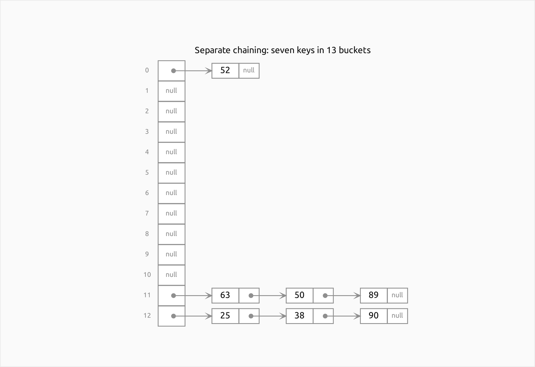
The picture is the chained table of the worked example, where three keys share bucket 11 and three share bucket 12. The invariant is simple: every node sits in the bucket of its key's hash, and no key appears twice. A chained table never fills up; its load factor can exceed 1, and α is then the mean chain length. Each node stores the key's hash code next to the key, so that a resize can move nodes without hashing any key again.

Open addressing and the search invariant

Open addressing stores every entry in the array itself, at most one per slot, so the load factor stays below 1. A key whose home slot h(k) is taken tries other slots in a fixed order, its probe sequence h(k, 0), h(k, 1), h(k, 2) and so on, where probe 0 is the home slot. The three classic strategies below differ only in that sequence.

• Insert follows the key's probe sequence to the first slot that holds no key and places it there.
• Search follows the same sequence and stops when it finds the key, or at the first empty slot, which proves the key absent.

Search is correct because of one invariant: every stored key can be reached from its home slot along its own probe sequence without passing an empty slot. Insertion keeps it, since a key is placed at the first free slot of its sequence and every slot before that was occupied. A search for a present key therefore meets it before any empty slot, and a search that reaches an empty slot can stop. open_addressing_violation checks exactly this, key by key, after every operation in the tests. Deletion is the operation that can break it, and the section on tombstones shows how to delete without doing so.

Linear probing

Linear probing tries the next slot, then the one after, wrapping from the last slot to the first:

The sequence visits every slot, so an insertion succeeds whenever any slot is free, and the slots it visits are neighbours in memory, which modern caches reward. Its weakness is primary clustering. Occupied slots form runs, and a key that hashes anywhere into a run has to walk to its end and then extends it by one. A run of length L is hit by L + 1 different home slots, so long runs catch more keys and grow faster than short ones, and two runs that touch merge into one. The worked example shows a run of seven slots forming from keys with three different homes.

Quadratic probing

Quadratic probing jumps further each time, so that keys colliding at one slot spread out instead of queueing behind each other:

The catch is that, unlike linear probing, the sequence need not visit every slot, and an insertion can fail although the table has free slots. With c1 = 0 and c2 = 1 and a table of 16 slots, the squares modulo 16 are only 0, 1, 4 and 9, so a key whose home is 3 can only ever reach slots 3, 4, 7 and 12. Two settings come with a guarantee.

The first is a prime size with the table at most half full. The first (m + 1)/2 probes of the sequence h + i² are then all different:

A prime that divides a product divides one of its factors, and both factors are positive and smaller than m. So the first (m + 1)/2 probes land in (m + 1)/2 different slots, and if the table holds at most (m − 1)/2 keys before an insertion, at least one of them is free. That is why the package's QuadraticProbing insists on a prime size and its tables default to a maximum load of one half. Beyond half full, a prime table can still fail: in a table of 7 slots, five keys sharing home 2 leave three slots free when the fifth one fails, because h + i² from 2 reaches only four slots.

The second setting is a power-of-two size with the triangular numbers 0, 1, 3, 6, 10, ... as offsets, which is c1 = c2 = 1/2. Each probe moves one slot further than the previous one, and the first 2^p probes visit every slot of a table of 2^p:

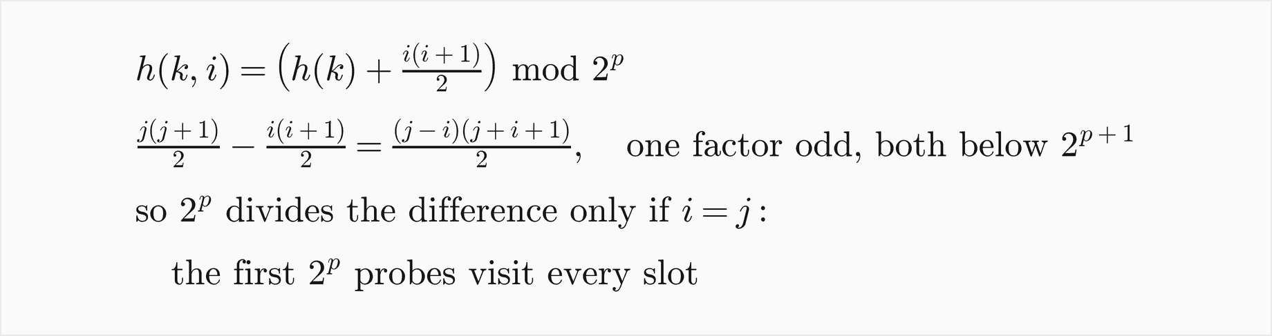
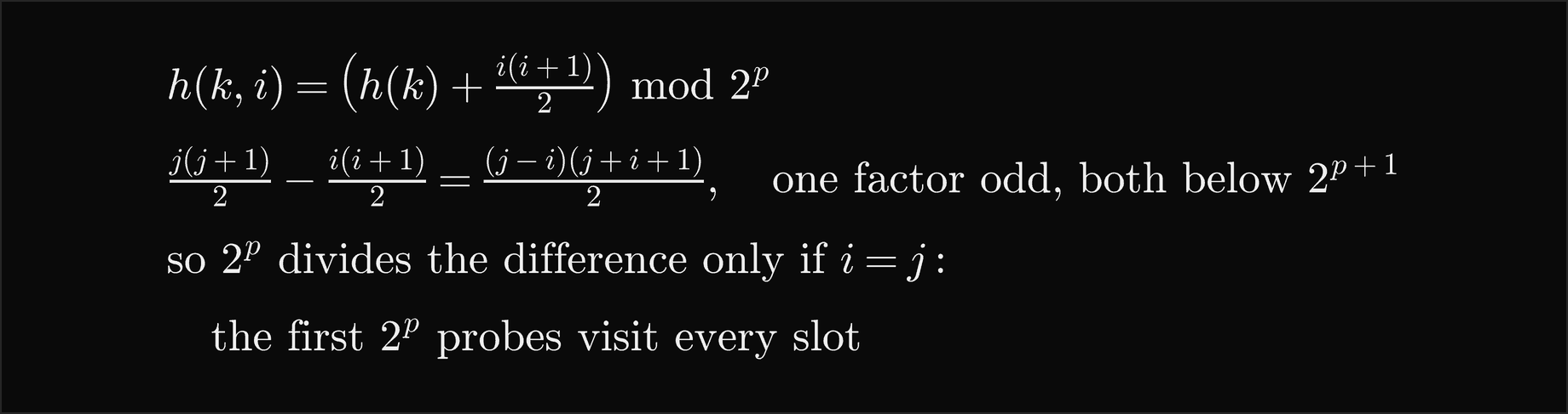
The two factors j − i and j + i + 1 add up to 2j + 1, an odd number, so one of them is odd. For the difference to be a multiple of 2^p, the product must be a multiple of 2^(p+1), and then the even factor alone must be, which is impossible for a positive number below 2^(p+1). TriangularProbing uses this form, steps through it with one addition per probe, and accepts any load below 1.

Quadratic probing removes primary clustering, since keys from neighbouring homes follow different paths, but not secondary clustering: two keys with the same home follow exactly the same sequence, so the k-th key with a given home pays for all k − 1 before it.

Double hashing

Double hashing derives the step from the key itself, with a second hash function:

Keys with the same home now take different steps and part after the first probe, so neither kind of clustering arises and the strategy behaves almost like the ideal of a random probe sequence for every key. Two conditions are essential. The step h2(k) must never be 0, or every probe lands on the home slot again; and it must share no factor with m, because the sequence then visits only m / gcd(h2(k), m) slots: a step of 4 in a table of 12 slots visits 3 of them. With a prime m any step from 1 to m − 1 qualifies, which gives the classic choice h2(k) = 1 + (k mod m′) for some m′ < m; with a power-of-two m, any odd step does. A second hash of the form k mod q is a trap, since it is 0 for every multiple of q. The package's DoubleHashing refuses a zero or non-coprime step with an error rather than looping, and its default step default_step uses the quotient k // m, the part of the code the home slot did not use, so that the two hashes are close to independent.

Deletion and tombstones

Deleting from a chained table is ordinary list surgery. In open addressing it is the subtle operation, because simply emptying the slot breaks the search invariant: every key whose probe path passed through that slot is now separated from its home by an empty slot, and searches for it stop early and report it missing.

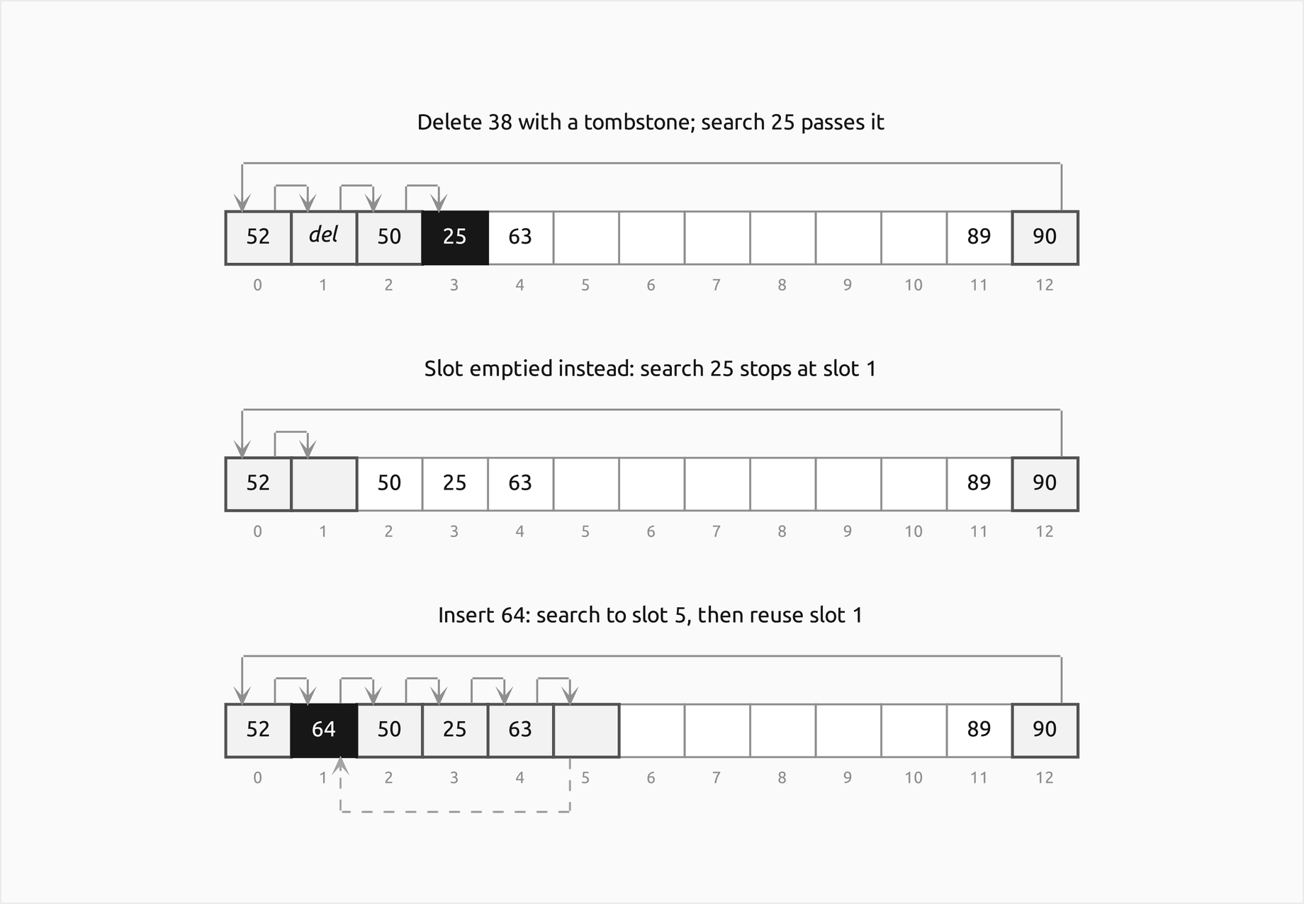
The standard fix is a tombstone, a marker that says "something was deleted here". A search treats a tombstone like an occupied slot that never matches and keeps going; only an empty slot ends it. An insertion may reuse the first tombstone on its path, but only after following the path to an empty slot to make sure the key is not already stored further along; placing it at the first tombstone without that check stores the key twice, as the third pitfall below shows. Tombstones have a price: a search walks over them as if they were keys, so for the cost of an unsuccessful search the relevant load is the number of keys plus tombstones over m. The package counts both and rebuilds the table when they fill it, which clears every tombstone.

Linear probing has an alternative without tombstones, Knuth's backward-shift deletion: empty the slot, then walk forward through the rest of the run and move back every entry whose home lies at or before the hole, since the hole is on that entry's own path; the hole moves to where the entry came from, and the walk ends at the first empty slot. The table is left exactly as if the key had never been inserted. BackwardShiftTable implements it, and the tests check that its occupied slots always equal those of a table built without the deleted keys.

Load factor, resizing and rehashing

Every cost below grows with the load factor, so a table must grow as keys arrive. The package's tables take a maximum load: when an insertion would push the number of used slots (keys plus tombstones) past it, the table rebuilds itself into a larger array before inserting. The new size is the next suitable size above twice the old one, a prime for division hashing and a power of two for triangular probing. Every live entry is reinserted into the new array, which is called rehashing, because its home slot k mod m changes with m. Copying entries to the same index in a larger array would leave nearly every key where its searches no longer look; in the worked example all seven keys are lost that way. A table whose slots are mostly tombstones is rebuilt at the same size, which is enough to clear them.

Shrinking is optional and needs a gap. A table that halves below some minimum load must choose that minimum well below half the maximum, or the load right after a doubling already lies below it, and a few deletions and insertions at the boundary make the table halve and double again and again; examples/resizing_and_deletion.py measures that thrashing. The cost section shows that doubling makes resizing cost O(1) amortized per insertion, while growing by a fixed number of slots does not.

Primary and secondary clustering

The two kinds of clustering are best seen side by side. The picture below inserts the same 96 random keys into tables of 128 slots with linear probing, quadratic probing with triangular numbers and double hashing.

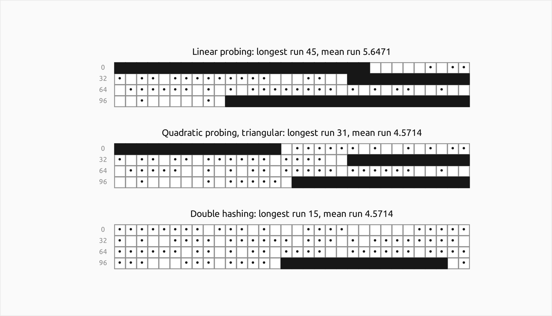
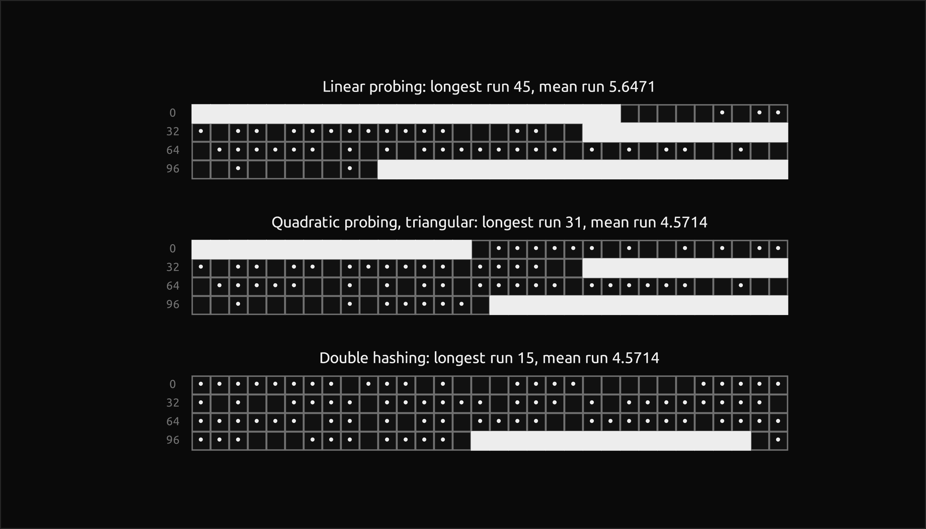
Linear probing merges its runs into long stretches, the longest covering 45 slots, a third of the table; a key that hashes anywhere into such a run pays for the rest of it. Quadratic probing and double hashing, at the same load of 0.75, leave mostly short runs. Secondary clustering is invisible in a single picture, since it concerns keys with the same home rather than neighbouring slots; the cost section measures it.

Cost

Every operation

With a hash function that behaves like random hashing and a load factor kept below a constant:

• search, insert and delete take O(1) expected time in every strategy; the constant depends on α and on the strategy, as derived below.
• the worst case of a single operation is Θ(n): all keys may hash to one slot, which happens with a bad hash function or with keys chosen by an adversary, the subject of Hashing in practice.
• an insertion that triggers a resize costs Θ(n) itself, but with doubling the resizes cost O(1) amortized per insertion.
• iteration costs Θ(m + n), since empty slots are visited too.
• nothing ordered is supported: the minimum, the successor of a key or a range of keys all cost Θ(n).

The distinction between expected, amortized and worst case matters more here than for most structures. Expected costs average over the randomness of the hash values, so they hold for typical keys but promise nothing for every input; amortized costs average over a sequence of operations and are guaranteed; a worst case bounds every single operation. A search tree gives O(log n) in the worst case; a hash table gives O(1) only on average, which is why systems with strict latency requirements, or keys that an attacker controls, pay attention to which they need.

All costs below count probes: the slots of the array an open-addressing search examines, including the empty slot that ends an unsuccessful search, and in chaining the bucket itself plus every node examined. A probe is one look at a place where the key might be, and so a fair unit for comparing the strategies.

Separate chaining

Under random hashing the expected length of the chain in the bucket of a missing key is exactly α, and an unsuccessful search reads the bucket and walks the whole chain:

A successful search for the key inserted i-th reads the bucket, then passes every key inserted later into the same bucket (new keys are linked at the head) and finally the key itself. Each of the n − i later keys is in the same bucket with probability 1/m:

Both grow only linearly with α, and a chained table works at any load; at α = 1 a missing key costs 2 probes and a present one 2.5. The extra 1 in the successful case is the price of the pointer: the bucket itself holds no key.

Uniform hashing

For open addressing the reference point is uniform hashing: every key's probe sequence is a random ordering of all m slots. An unsuccessful search needs a probe i exactly when the first i − 1 probes all found used slots:

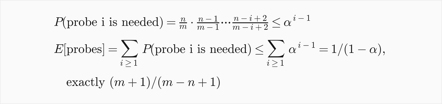
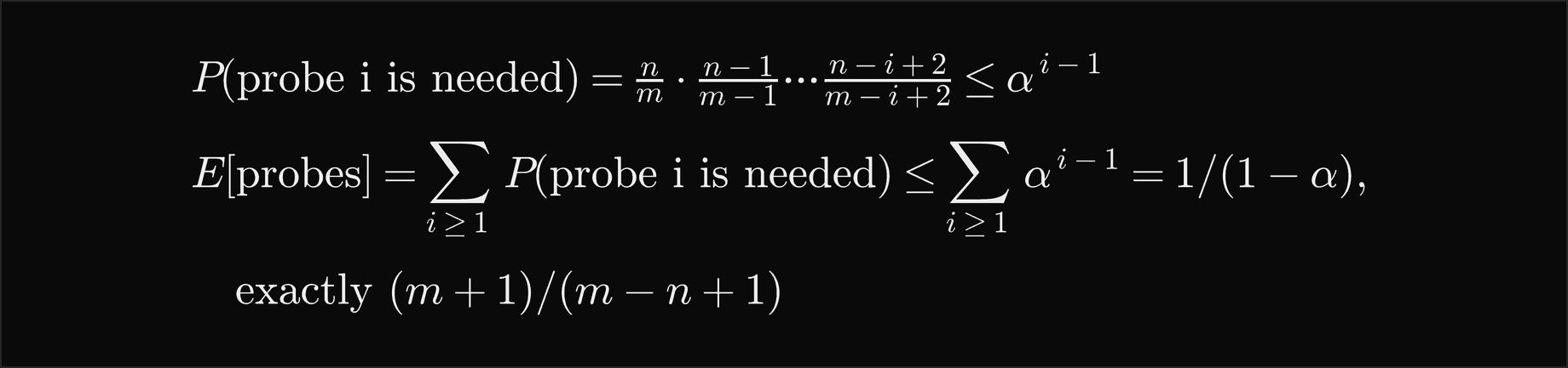
The expected count of a positive integer is the sum of the probabilities that it is at least i, and the geometric series gives 1/(1 − α): 2 probes at half load, 10 at α = 0.9. The exact value for m slots and n keys is (m + 1)/(m − n + 1), which the tests check by enumerating every possible probe sequence of small tables.

Successful searches retrace insertions

Without deletions, a search for a present key follows the same probe sequence as the insertion that placed it, and that insertion was an unsuccessful search in the table as it was then. If C′(α) is the expected cost of an unsuccessful search at load α, the expected cost C(α) of a successful search is the average of C′ over the loads at which the keys were inserted:

This turns every unsuccessful formula into a successful one. For uniform hashing:

That is 1.3863 probes at half load and 2.5584 at α = 0.9: a present key is cheap even when a missing one is not, because most keys were inserted while the table was emptier.

Linear probing: Knuth's formulas

Linear probing is not uniform hashing, because its probe sequences are not independent, and its analysis, first done by Knuth in 1963, is harder. A short derivation uses a picture that makes the table infinite: slot j receives X_j keys, independent Poisson variables with mean α, and keys that find their slot taken are carried to the right.

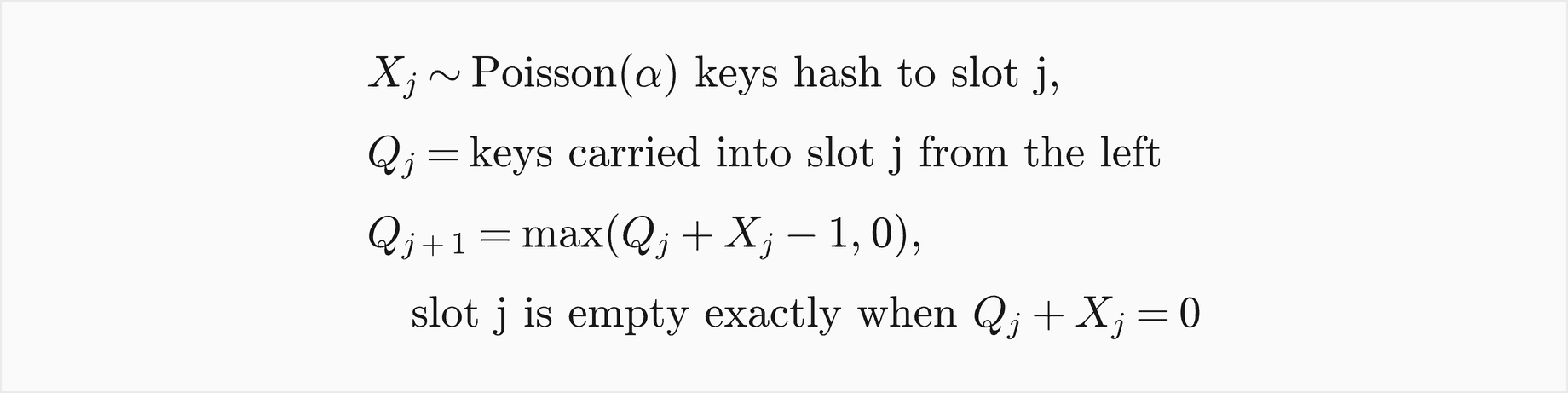
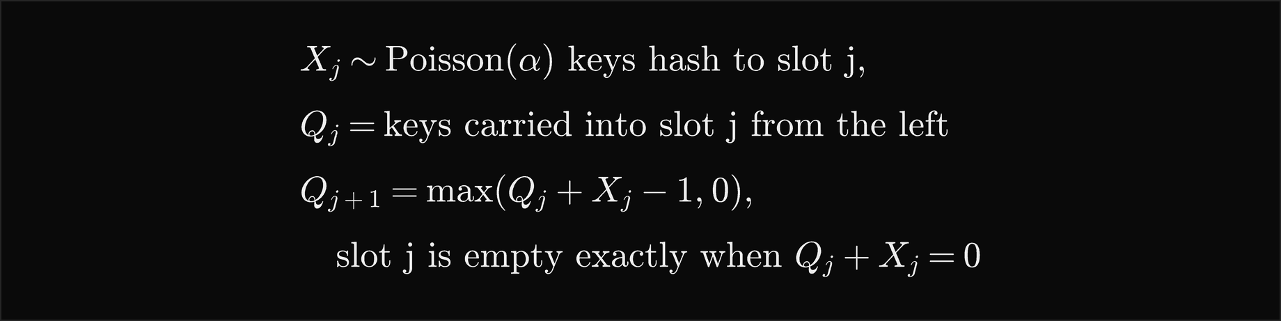
Each slot takes one of the keys that reach it, so the backlog Q behaves like the queue of a server that serves one customer per time step. In the steady state its distribution does not change from one slot to the next, which gives two equations. Taking expectations of the recurrence shows that a fraction 1 − α of the slots is empty, as it must be. Squaring the recurrence before taking expectations gives the mean backlog:

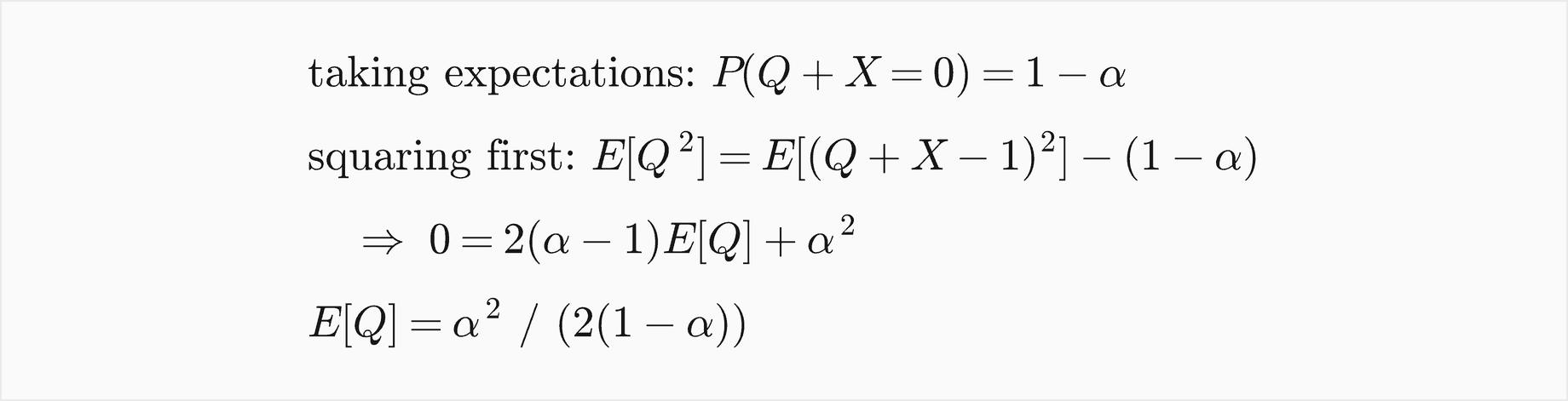
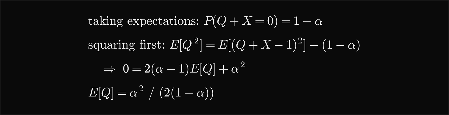
(When Q + X = 0 the square of Q + X − 1 is 1 while the new backlog is 0, which is where the term 1 − α comes from.) An unsuccessful search starting at slot 0 meets B_0 = Q_0 + X_0 keys that need slots from 0 on, and the run of used slots ends when that backlog first drops to zero. Each further slot takes one key and brings X new ones, so the backlog falls by 1 − α per slot on average:

This is Wald's identity for a random walk with drift −(1 − α). Counting the empty slot that ends the search, and using E[B_0] = E[Q] + α, gives Knuth's formula for an unsuccessful search:

The averaging integral then gives the successful search:

The square is primary clustering in a formula. At half load a missing key costs 2.5 probes against 2 for uniform hashing, but at α = 0.9 it costs 50.5 against 10. A present key costs 1.5 and 5.5. Knuth also found the exact expectation for m slots and n keys, as sums that the package evaluates in linear_exact:

The tests check these sums against an enumeration of every possible sequence of home slots for tables of up to 7 slots, and check that they approach the asymptotic formulas for large tables.

The same picture gives the length of the runs. A run starts at slot j when slot j − 1 is empty and slot j is not; an empty slot passes no backlog on, so slot j is then used exactly when X_j ≥ 1:

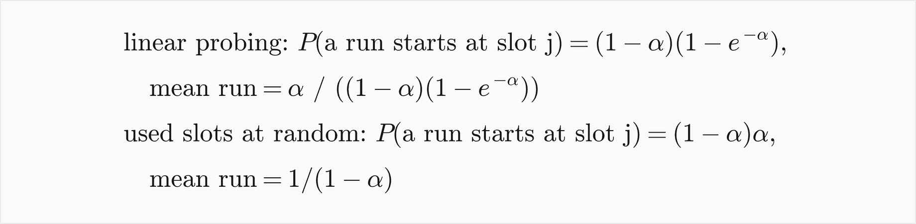
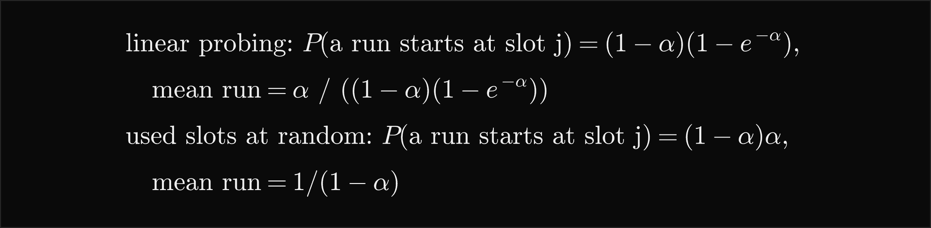
At α = 0.9 a run of used slots is 15.1661 slots long on average under linear probing, against 10 when the same number of used slots is scattered at random.

Quadratic probing and secondary clustering

No exact formula is known for quadratic probing, but Knuth's estimates for an idealized method with secondary clustering only, where keys with the same home share their sequence and nothing else interferes, describe it well:

At half load these give 2.1931 and 1.4431 probes, a little above uniform hashing, and at α = 0.9 they give 11.4026 and 2.8526, far below linear probing. The successful formula is again the average of the unsuccessful one, which the tests check by numerical integration.

Counted probes

The example probes_and_clustering.py fills tables of 8191 slots (8192 for triangular probing) with random keys, and at every load from 0.1 to 0.95 counts the probes of searching for every stored key and for 4000 absent ones, averaged over five seeds.

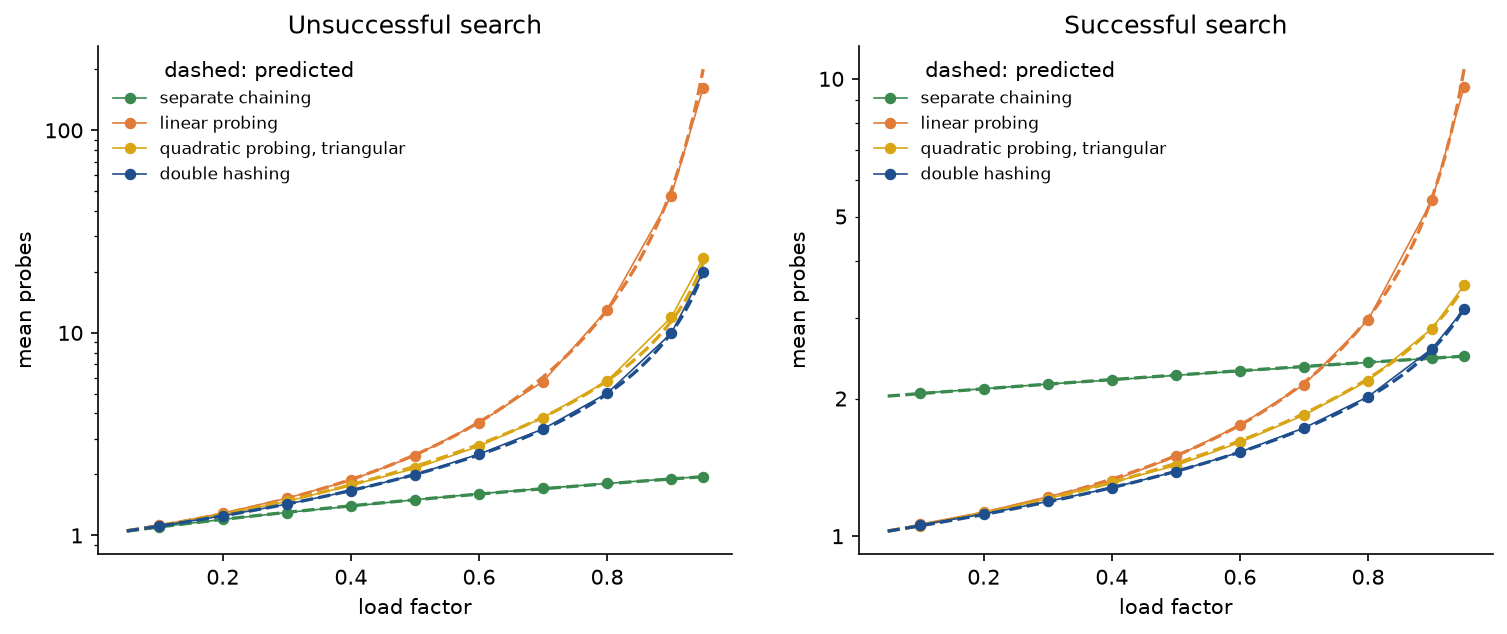
Every measured curve lies on its prediction up to α = 0.9. At half load chaining made 1.5007 probes per missing key and 2.2479 per present key against 1.5 and 2.25; linear probing 2.4777 and 1.4938 against 2.5 and 1.5; double hashing 1.9956 and 1.3848 against 2.0 and 1.3864. Quadratic probing sits a little below Knuth's estimate with prime sizes (2.1281) and close to it with triangular numbers (2.1406, against 2.1931). At α = 0.9 the differences between strategies are large: a missing key costs 1.9070 probes with chaining, 9.9387 with double hashing, 11.9167 with triangular quadratic probing and 47.3470 with linear probing, against Knuth's 50.5122. The asymptotic formula for linear probing is approached slowly near a full table. For 8191 slots Knuth's exact sums give 48.9521 at 0.9 and 177.3729 at 0.95, against 50.5122 and 200.0612 asymptotically; the measured mean at 0.95, 162.0026, comes from five tables that individually gave between 115 and 235, because a single long run decides the cost of a nearly full table.

The conclusion for practice: chaining is the most forgiving at high load; double hashing is the most economical open addressing; linear probing is excellent up to about half or two thirds full, where its cache-friendly sequential probes more than pay for the extra probes, and terrible near full.

Clustering measured

The same example measures both kinds of clustering.

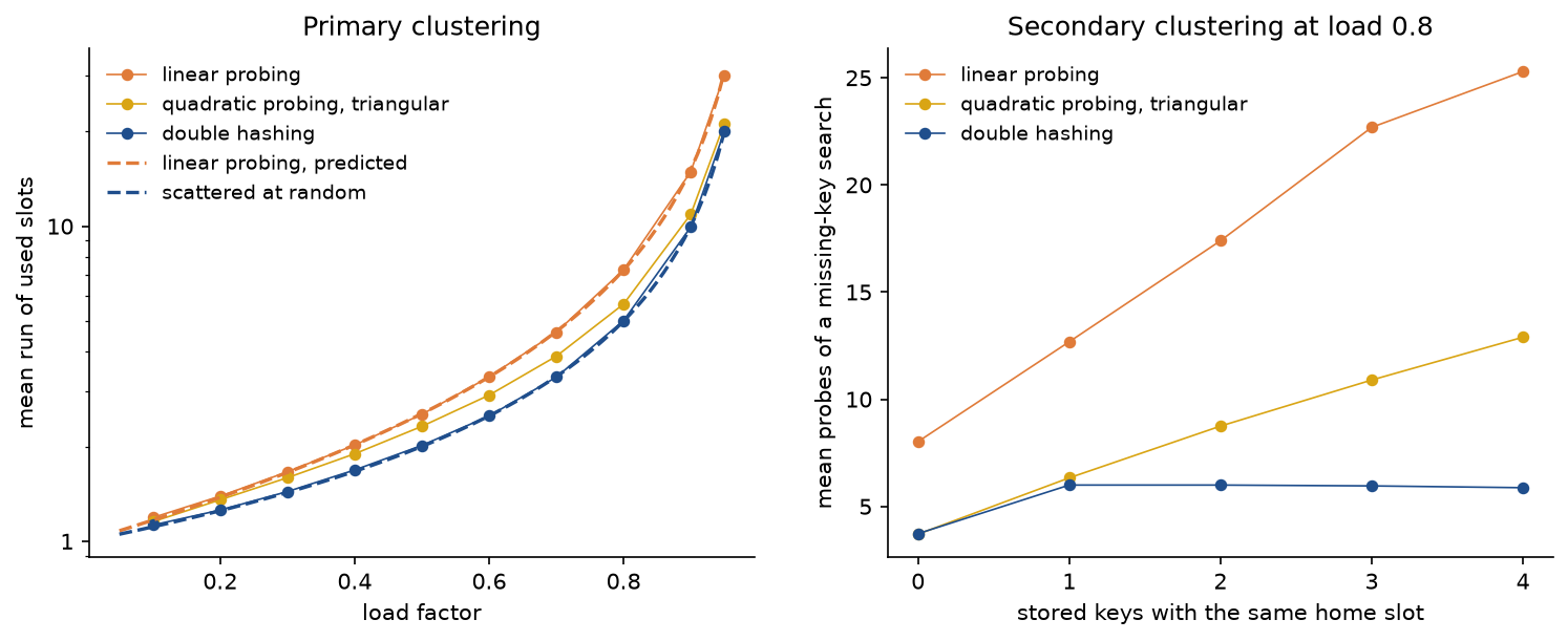
Primary clustering is the gap in the left panel. At half load the mean run under linear probing was 2.5277 slots against the predicted 2.5415, and under double hashing 2.0140 against 2.0000 for used slots scattered at random; quadratic probing, at 2.3159, has a little local clustering left, because its first step always goes to the next slot. Secondary clustering is the slope in the right panel. A missing key whose home is shared by k stored keys must pass at least k slots under quadratic probing, since those keys sit on its own sequence: the mean cost rose from 3.7047 probes with no shared home to 6.3338, 8.7489, 10.9002 and 12.8971 with one to four. Under double hashing it was 3.7291 with none and 5.9978, 5.9974, 5.9584 and 5.8750 with one to four: once the home slot is known to be taken, the number of keys behind it does not matter, because they all left along different steps.

The amortized cost of growth

A table that doubles when it reaches its maximum load rebuilds rarely and expensively. The rebuild that happens when the table holds k keys moves all k of them, and the rebuilds before it moved at most half as many each, so the total over n insertions is a geometric series; growing by a fixed number c of slots instead rebuilds every αc insertions:

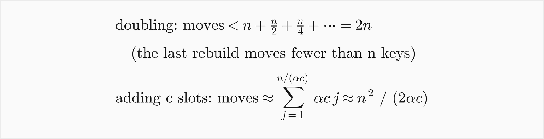
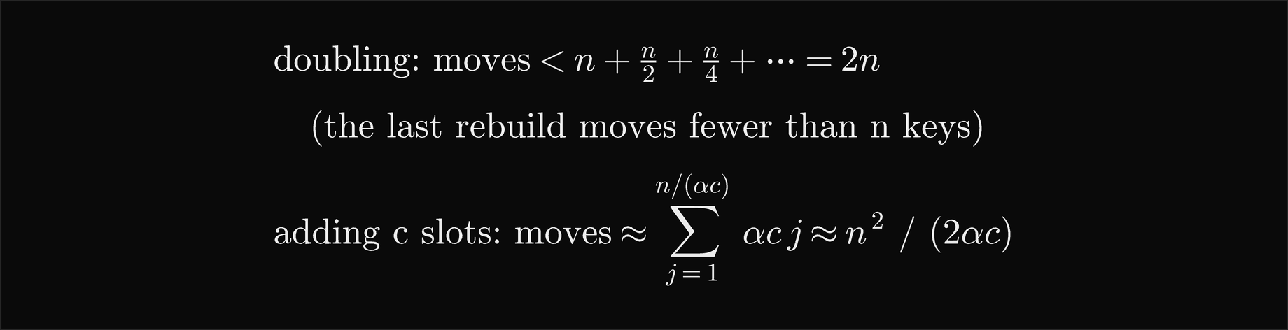
So doubling costs fewer than two moves per insertion on top of the insertion's own probes, O(1) amortized, while a fixed increment costs Θ(n) per insertion on average. The aggregate argument is the one Amortized analysis makes for dynamic arrays, and the potential method gives the same bound. The example resizing_and_deletion.py inserts 20000 random keys into linear-probing tables that start with 11 slots and a maximum load of 0.5.

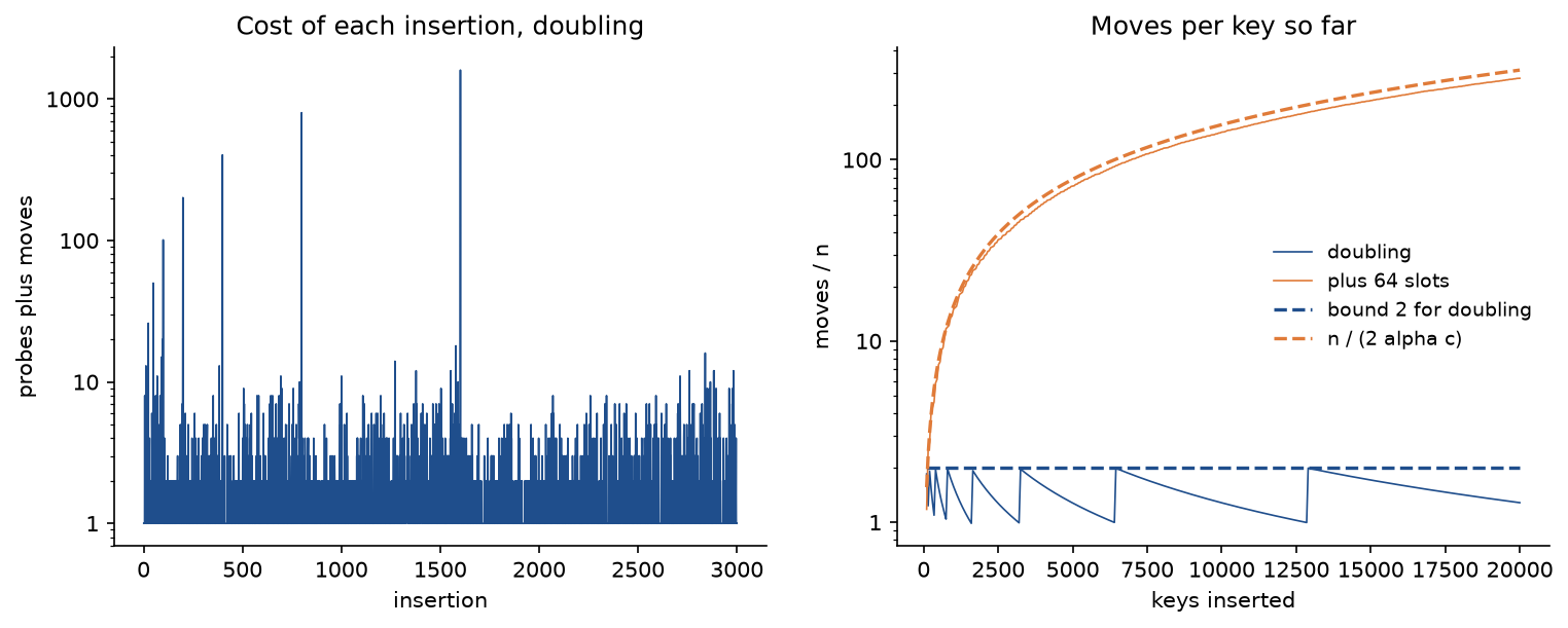
Doubling made 12 rebuilds and 25674 moves in all, 1.2837 per key, below the bound of 2, although the most expensive single insertion paid 12862 probes and moves. Growing by 64 slots made 567 rebuilds and 5632777 moves, 281.6388 per key, near the prediction of n/(2αc) = 312.5 (the prime sizes grow by slightly more than 64 each time). For a table that also shrinks, the same example shows why the minimum load must sit well below half the maximum: right after the seventh doubling, deleting two keys and inserting two, 200 times, caused 400 rebuilds and 204600 moves when the table halved below half its maximum load, and none when it halved below a quarter.

Tombstones over time

Tombstones make deletions cheap but leave debt behind. The example keeps 254 keys in a linear-probing table of 509 slots and replaces one random key by a new one 6000 times, measuring missing-key searches as it goes.

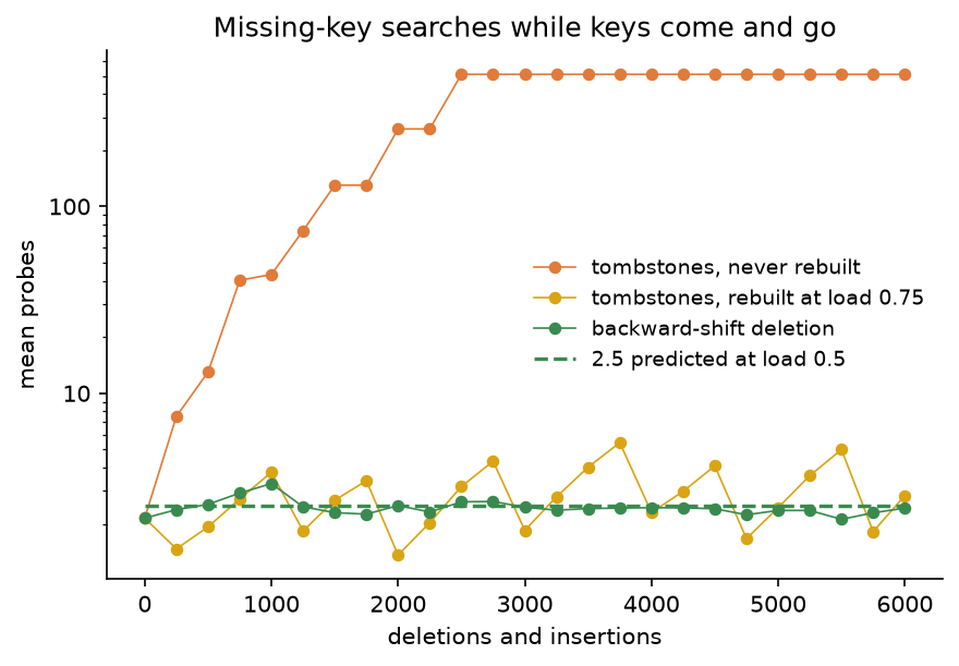
Without rebuilds, each deletion leaves a tombstone and each insertion reuses one only if its path happens to meet one before an empty slot, so tombstones accumulate until no empty slot is left: after 3000 operations every missing-key search walked all 509 slots. With rebuilds whenever keys and tombstones fill three quarters of the table, the first rebuild doubles it to 1019 slots, because half of it is live, and the six after it keep that size and only clear tombstones; the cost oscillates between clean and dirty. Backward-shift deletion keeps the table as if the deleted keys had never existed, and its cost stayed at 2.4300 after 6000 operations, Knuth's 2.5 for half load.

Worked example

Every step below is printed by examples/worked_example.py and asserted by tests/test_worked_example.py. The keys are the seven integers 52, 90, 89, 38, 50, 25 and 63, inserted in that order into tables of m = 13 slots with h(k) = k mod 13. They were chosen so that collisions happen: three of them share home 11 and three share home 12.

Hashing the keys

The home slots and, for double hashing, the steps h2(k) = 1 + (k mod 11):

• 52: 52 mod 13 = 0, step 1 + 8 = 9.
• 90: 90 mod 13 = 12, step 1 + 2 = 3.
• 89: 89 mod 13 = 11, step 1 + 1 = 2.
• 38: 38 mod 13 = 12, step 1 + 5 = 6.
• 50: 50 mod 13 = 11, step 1 + 6 = 7.
• 25: 25 mod 13 = 12, step 1 + 3 = 4.
• 63: 63 mod 13 = 11, step 1 + 8 = 9.

The steps lie between 1 and 11, never 0, and every one is coprime with the prime 13. For comparison, the multiplication method with m = 16 puts 52 in slot 2, since frac(52 · 0.6180339887) = 0.1378 and 16 · 0.1378 = 2.2043, and the seven keys in slots 2, 9, 0, 7, 14, 7 and 14.

For strings, take the anagrams spare, pears, reaps and parse. Their character codes sum to 539 for all four, so the character-sum hash puts them all in slot 539 mod 13 = 6. The polynomial hash with base 31, computed modulo 13 by Horner's rule, separates them. For spare, with the codes s = 115, p = 112, a = 97, r = 114 and e = 101:

• 115 mod 13 = 11.
• (11 · 31 + 112) mod 13 = 453 mod 13 = 11.
• (11 · 31 + 97) mod 13 = 438 mod 13 = 9.
• (9 · 31 + 114) mod 13 = 393 mod 13 = 3.
• (3 · 31 + 101) mod 13 = 194 mod 13 = 12.

So spare goes to slot 12, and in the same way pears goes to 0, reaps to 5 and parse to 7.

Separate chaining insert by insert

Each insertion reads the bucket and walks its chain to check for the key, then links the new node at the head:

• 52: bucket 0 is empty; link 52. One probe.
• 90: bucket 12 is empty; link 90. One probe.
• 89: bucket 11 is empty; link 89. One probe.
• 38: bucket 12 holds 90, not 38; link 38 before it. Two probes.
• 50: bucket 11 holds 89; link 50 before it. Two probes.
• 25: bucket 12 holds 38 and 90; link 25 at the head. Three probes.
• 63: bucket 11 holds 50 and 89; link 63 at the head. Three probes.

The chains are 52 in bucket 0, 63 → 50 → 89 in bucket 11 and 25 → 38 → 90 in bucket 12, after 13 probes in all. Searching for 90 reads bucket 12 and passes 25 and 38 before finding it, 4 probes; searching for the absent 77, whose home is also 12, walks the same chain to its end, 4 probes as well.

Linear probing insert by insert

Each insertion tries the home slot and then the following slots, wrapping from 12 to 0:

• 52: slot 0 is empty; place it. One probe.
• 90: slot 12 is empty; place it. One probe.
• 89: slot 11 is empty; place it. One probe.
• 38: slot 12 holds 90 and slot 0 holds 52; slot 1 is empty; place it. Three probes.
• 50: slots 11, 12, 0 and 1 hold 89, 90, 52 and 38; slot 2 is empty; place it. Five probes.
• 25: slots 12, 0, 1 and 2 hold 90, 52, 38 and 50; slot 3 is empty; place it. Five probes.
• 63: slots 11, 12, 0, 1, 2 and 3 are all taken; slot 4 is empty; place it. Seven probes.

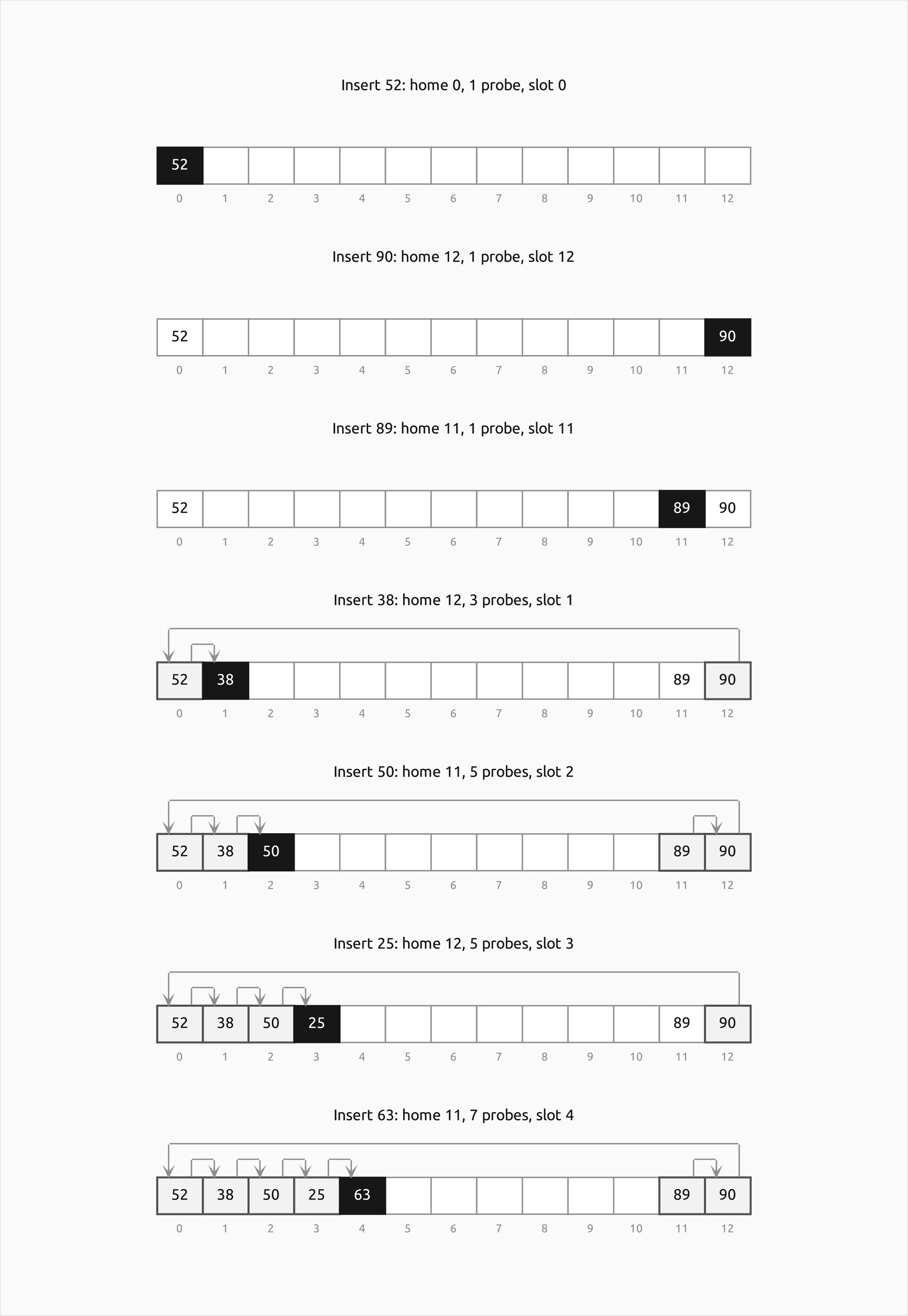
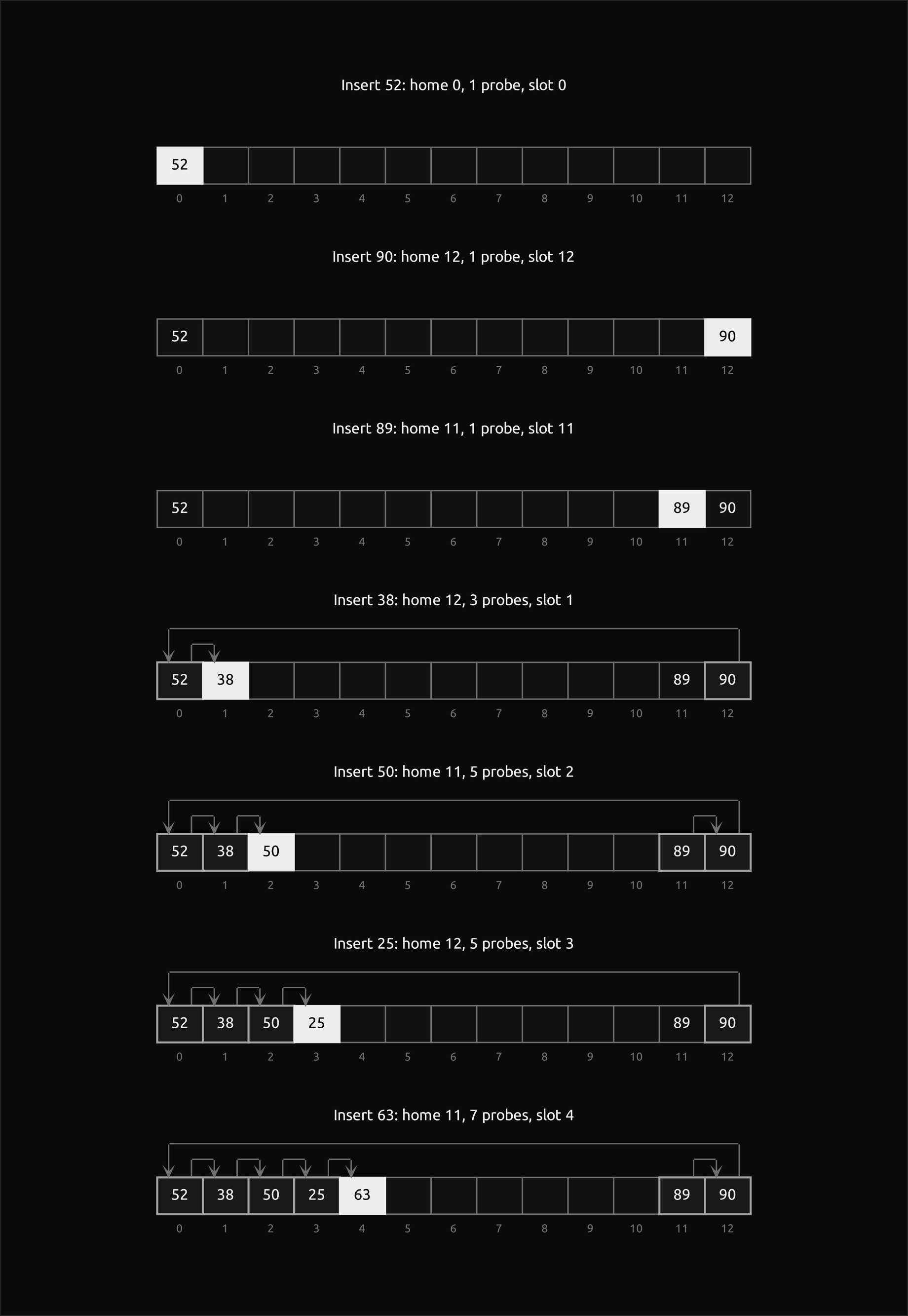
The table ends as 0: 52, 1: 38, 2: 50, 3: 25, 4: 63, 11: 89, 12: 90, after 23 probes. All seven keys form one run from slot 11 around to slot 4, and 52, whose home 0 was free when it arrived, now sits in the middle of it: every later key from homes 11 and 12 had to walk past it. That is primary clustering in miniature.

Quadratic probing insert by insert

The probes are h(k) + i² modulo 13, that is home, home + 1, home + 4, home + 9 and so on:

• 52, 90 and 89 find their homes 0, 12 and 11 empty. One probe each.
• 38: slot 12 holds 90, slot 13 mod 13 = 0 holds 52, slot 16 mod 13 = 3 is empty; place it. Three probes.
• 50: slot 11 holds 89, slot 12 holds 90, slot 15 mod 13 = 2 is empty; place it. Three probes.
• 25: slots 12, 0 and 3 hold 90, 52 and 38; slot 21 mod 13 = 8 is empty; place it. Four probes.
• 63: slots 11, 12 and 2 hold 89, 90 and 50; slot 20 mod 13 = 7 is empty; place it. Four probes.

The table ends as 0: 52, 2: 50, 3: 38, 7: 63, 8: 25, 11: 89, 12: 90, after 17 probes, and its longest run is 3. Notice 25 retracing every step of 38, and 63 every step of 50: keys with the same home follow the same path, which is secondary clustering. The table holds 6 keys before the last insertion, at most (13 − 1)/2, so the guarantee of the prime size applied to every insertion.

Double hashing insert by insert

The probes are h(k) + i · h2(k) modulo 13:

• 52, 90 and 89 find their homes empty. One probe each.
• 38, step 6: slot 12 holds 90, slot 18 mod 13 = 5 is empty; place it. Two probes.
• 50, step 7: slot 11 holds 89, slot 5 holds 38, slot 25 mod 13 = 12 holds 90, slot 32 mod 13 = 6 is empty; place it. Four probes.
• 25, step 4: slot 12 holds 90, slot 16 mod 13 = 3 is empty; place it. Two probes.
• 63, step 9: slot 11 holds 89, slot 20 mod 13 = 7 is empty; place it. Two probes.

The table ends as 0: 52, 3: 25, 5: 38, 6: 50, 7: 63, 11: 89, 12: 90, after 13 probes. The three keys with home 12 left along steps 3, 6 and 4, and the three with home 11 along steps 2, 7 and 9.

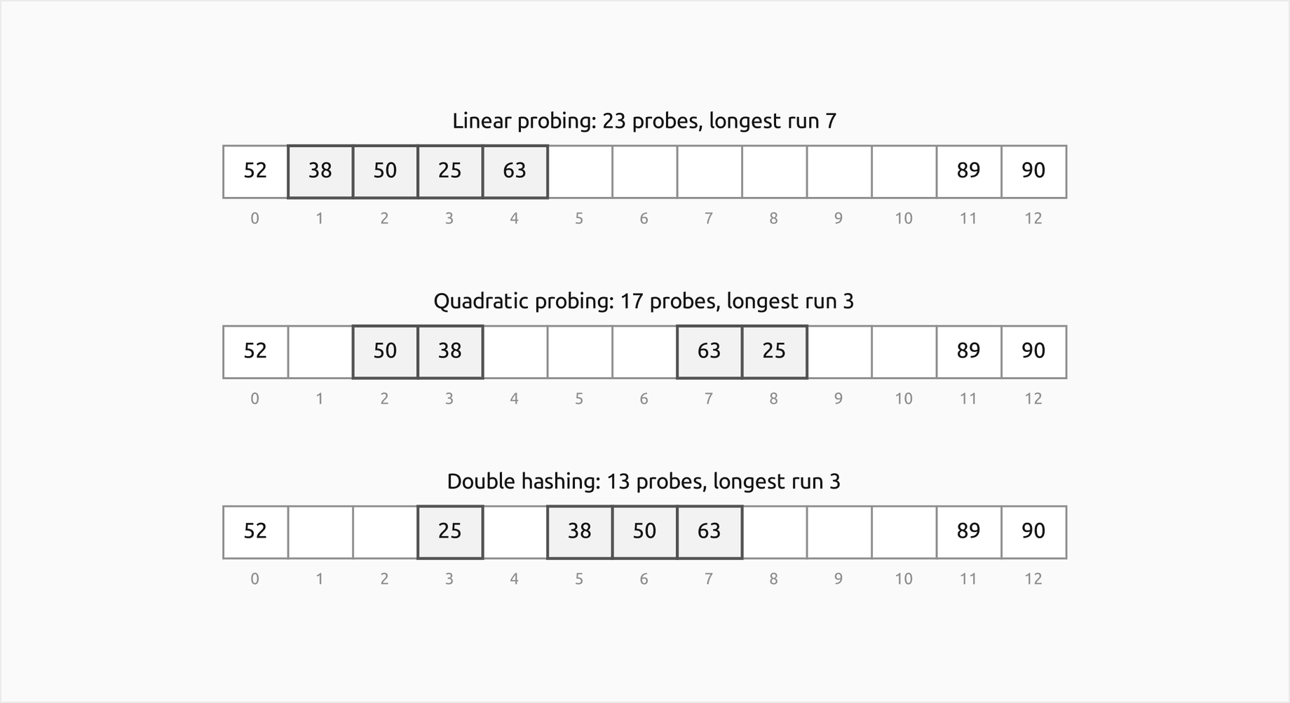
Side by side, the three tables hold the same keys at the same load of 7/13 = 0.5385 with 23, 17 and 13 probes. The ordering is the one the cost section predicts for large tables, though seven keys are too few for the counts themselves to mean much.

Searching for a missing key

A search for 77, whose home is 12, ends at the first empty slot of its sequence:

• Separate chaining: bucket 12 and its three nodes, 4 probes.
• Linear probing: slots 12, 0, 1, 2, 3 and 4 are taken and slot 5 is empty, 7 probes.
• Quadratic probing: slots 12, 0, 3, 8, then 12 + 16 = 28 → 2 and 12 + 25 = 37 → 11 are taken, and 12 + 36 = 48 → 9 is empty, 7 probes.
• Double hashing: the step of 77 is 1 + (77 mod 11) = 1, so its sequence happens to be the linear one; slots 12 and 0 are taken and slot 1 is empty, 3 probes.

Deleting with a tombstone

Delete 38 from the linear-probing table. The search finds it at slot 1 after probing slots 12, 0 and 1, and replaces it with a tombstone. Then:

• Search 25: slot 12 holds 90, slot 0 holds 52, slot 1 holds a tombstone and the search keeps going, slot 2 holds 50, slot 3 holds 25. Found after 5 probes.
• Had slot 1 been emptied instead, the same search would stop there after 3 probes and report 25 missing, although 25, 50 and 63 are all still in the table.
• Insert 64, whose home is 12: slots 12 and 0 are taken, slot 1 holds the tombstone, which the insertion remembers, slots 2, 3 and 4 hold 50, 25 and 63, and slot 5 is empty, which proves 64 absent. Then 64 goes into slot 1, the first tombstone on its path. Seven probes; the table again holds 7 keys and no tombstone.

With backward-shift deletion instead of a tombstone, deleting 38 empties slot 1 and then moves 50, 25 and 63 back one slot each, since each one's home (11, 12 and 11) lies at or before the hole: the table becomes 0: 52, 1: 50, 2: 25, 3: 63, 11: 89, 12: 90 after 3 moves.

Growing the table

The table was built with a maximum load of 0.6. Inserting 47 probes its home 47 mod 13 = 8, which is empty, but filling it would make 8 of 13 slots used, 0.6154, above the maximum. So the table first grows to the next prime above 2 · 13, which is 29, and reinserts its seven keys in slot order, each at its new home k mod 29, all of them free:

• 52 → 23, 64 → 6, 50 → 21, 25 → 25, 63 → 5, 89 → 2 and 90 → 3.

Then 47 probes its new home 47 mod 29 = 18, which is empty, and goes there. The insertion cost 2 probes and 7 moves, the load is now 8/29 = 0.2759, and the run of seven has dissolved into runs of at most two.

The code

The package hash_tables is plain Python, one idea per module. Importing it needs only the standard library; Matplotlib is imported by plotting.py alone.

• hash_functions.py holds the division and multiplication methods (in exact integer arithmetic), the polynomial and character-sum string hashes, hash_code, which every table uses, and mixed_hash_code, which scatters neighbouring codes.
• distribution.py measures how a function spreads keys over buckets (empty buckets, longest chain, colliding pairs, chi-squared) and holds the expectations under random hashing; primes.py finds prime and power-of-two sizes.
• probing.py holds the probing strategies LinearProbing, QuadraticProbing, TriangularProbing and DoubleHashing, each a sequence of slots with the size it needs, and default_step, a second hash that is never zero and always coprime with the size.
• chaining.py holds ChainedHashTable; slots.py the empty and tombstone markers and the entries of open addressing; open_addressing.py holds OpenAddressingTable for any probing strategy, with tombstones and resizing; backward_shift.py holds BackwardShiftTable, linear probing without tombstones.
• resizing.py chooses the size of a rebuilt table and holds the arithmetic of the amortized cost; hash_set.py turns any table into a set with the full set algebra.
• dictionary.py holds the simple implementations of the abstract data type that hash tables are measured against: PairList, SortedPairs and DirectAddressTable.
• expected_costs.py holds every formula of the cost section, including Knuth's exact sums; measurement.py fills tables to given loads and counts the probes of searches; clustering.py measures runs of used slots and the cost of shared homes.
• counting.py holds OperationCounter, with the fields hashes, probes, comparisons, moves and resizes that every table keeps, and CountedKey, which counts the hash codes and equality tests Python's dict asks for.
• trace.py holds the Step record that every operation can append to a trace list, and format_trace, which turns steps into the lines printed above.
• invariants.py holds hash_table_violation, is_hash_table and check_hash_table, which tests run after every operation of long random operation sequences.
• workloads.py holds the worked example's keys and seeded random inputs; layout.py places every slot, bucket and probe arrow, and drawing.py, chain_drawing.py and occupancy_drawing.py turn those positions into pinned Graphviz text for tables with their probe arrows, chained tables and occupancy pictures; comparisons.py puts dict, set and collections.Counter next to the package; pitfalls.py holds deliberately broken versions for the pitfalls below; plotting.py draws every figure in the handbook's colours.

Counting and tracing never change what the code does. The search at the heart of open addressing is one loop over the probe sequence:

first_free = None
for i, slot in enumerate(self.probing.sequence(code, self.size)):
    self.counter.probes += 1
    item = self.slots[slot]
    if item is EMPTY:
        record(trace, "probe-empty", key, slot, i)
        return None, slot if first_free is None else first_free
    if item is TOMBSTONE:
        record(trace, "probe-tombstone", key, slot, i)
        if first_free is None:
            first_free = slot
        continue
    self.counter.comparisons += 1
    if item.key == key:
        record(trace, "probe-match", key, slot, i, item.key)
        return slot, None
    record(trace, "probe-other", key, slot, i, item.key)
return None, first_free

The examples run in a few seconds each from the repository root:

• examples/worked_example.py prints every step of the worked example and writes the four generated diagram sources of the worked example.
• examples/hash_function_quality.py measures how evenly hash functions spread strided integers, random integers and words, and the first collision.
• examples/probes_and_clustering.py counts probes for every strategy against the predictions, measures both kinds of clustering and writes the clustering diagram source.
• examples/resizing_and_deletion.py measures the amortized cost of growth, thrashing and tombstones over time.
• examples/common_mistakes.py runs every broken version from pitfalls.py next to the correct code.
• examples/compare_with_dict.py checks every table against dict, set and Counter, counts what dict asks of its keys and compares the dictionary implementations.
• examples/practice.py prints fresh exercises with their solutions; --seed gives a new set.

python hashing/hash-tables/examples/worked_example.py
python hashing/hash-tables/examples/hash_function_quality.py
python hashing/hash-tables/examples/probes_and_clustering.py
python hashing/hash-tables/examples/resizing_and_deletion.py
python hashing/hash-tables/examples/common_mistakes.py
python hashing/hash-tables/examples/compare_with_dict.py
python hashing/hash-tables/examples/practice.py --seed 7

The sample project, project/spell_checker.py with its helpers project/corpus.py and project/spelling.py, is a spell checker and word-frequency counter for a public-domain novel, built entirely on the package's tables. It downloads The Adventures of Sherlock Holmes and the 113809-word crossword list of the Moby word lists once into .data/hash-tables, loads the list (plus the one-letter words a and i, which crossword lists leave out) into a HashSet, counts the words of the book in an OpenAddressingTable and reports the words the list does not know. A word that never appears in lower case is taken as a name; for the others it suggests the known words one edit away (one letter deleted, swapped with its neighbour, replaced or inserted), the ones the book uses most first. It then makes 2000 seeded typos of book words to measure the suggestions, measures the probes of every collision strategy on the real words at four load factors, and checks every answer against Python's set, dict and Counter. Options --strategy, --loads, --bits, --typos, --show, --seed and --strict change the run, and --figures writes the PNGs elsewhere; the default run takes about 5 seconds after the download.

python hashing/hash-tables/project/spell_checker.py
python hashing/hash-tables/project/spell_checker.py --strategy double --loads 0.5,0.7,0.8,0.9,0.95

The default run splits the book into 105301 tokens, leaves 199 contractions such as don't unchecked because the list has none, and counts 105102 words, 7803 of them different; the most frequent are the (5630), and (3018) and i (3003). The list lacks 596 of the different words: 376 are only ever capitalised and taken as names, such as Holmes and Lestrade, and 220 others include stepfather and waistcoat, which the list does not have, and neighbourhood and endeavoured, for which it suggests the spellings neighborhood and endeavored. On the 2000 typos, the first suggestion was the intended word 0.8710 of the time, from 5.7515 suggestions on average, and the intended word was always among them. Counts, memberships and suggestions all agreed with Counter and set.

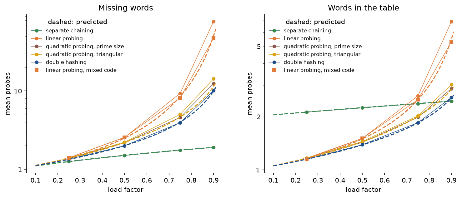
On real words the strategies behave as on random keys, with one instructive exception. Chaining, quadratic probing and double hashing match their predictions; double hashing at α = 0.9 made 10.1058 probes per missing word against 10.0002. Linear probing made 77.1584 against 50.5015, half as many again. The reason is the polynomial hash itself: words that differ only in their last letter get codes a few units apart, and so homes a few slots apart, which is exactly the input primary clustering feeds on. In the list, 28203 of the 113811 words share all but their last letter with another word; base, bash, bask, bass and bast land in slots 2435, 2438, 2441, 2449 and 2450 of 65521. Chaining does not care where neighbouring buckets are, and double hashing gives each of these words its own step. Mixing the code before reducing it, by multiplying it by Knuth's 64-bit golden-ratio constant and keeping the high bits (mixed_hash_code), scatters such families, and linear probing then made 47.4554 probes, back on Knuth's curve. Linear probing needs more from its hash function than the other strategies do, and the theory agrees: its expected constant cost is guaranteed for hash functions drawn from a 5-wise independent family but not for every 4-wise independent one, while chaining needs only pairwise independence.

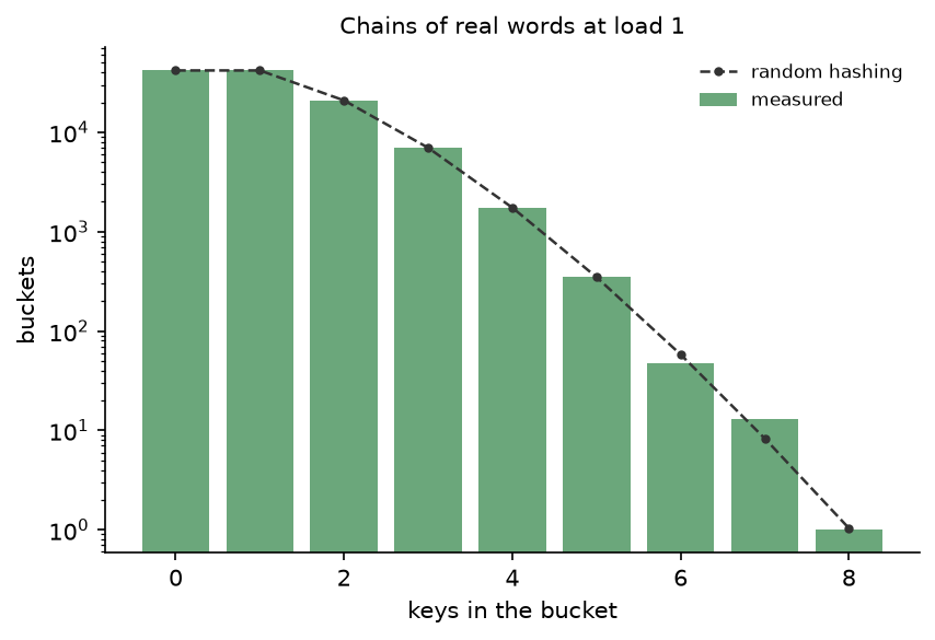
Chained at load 1, the real words fill buckets like balls thrown at random: 41811 empty buckets against 41874.4293 expected, 42049 with one word against 41871.8540, 20759 with two against 20934.4554, and one bucket of eight against 1.0378.

The notebook hash_tables.ipynb follows this page: the worked example step by step, the diagrams, the distributions, the counted probes against their predictions, clustering, growth and tombstones, the comparison with dict and set, and the project's spell checker on a few words. The tests in tests check the worked example value by value, the invariants after thousands of random operations, the exact formulas against exhaustive enumeration, the measured probes against the predictions, and the agreement with dict, set and Counter, and run in a few seconds:

python -m pytest hashing/hash-tables

The examples and tests use only synthetic data generated from seeds by workloads.py. The project downloads two texts from Project Gutenberg into .data/hash-tables at the repository root, which is never committed: The Adventures of Sherlock Holmes by Arthur Conan Doyle (eBook 1661), in the public domain in the United States, and the crossword list crosswd.txt of Grady Ward's Moby word lists (eBook 3201), which its author placed in the public domain; both files are distributed under the Project Gutenberg License, which permits this use. Project Gutenberg regenerates its files from time to time, so the project pins the SHA-256 of the text between the start and end markers rather than of the whole file, warns when the text differs, and stops only with --strict.

In practice

Python's dict and set

Python's dict and set are hash tables with open addressing, written in C. The package's tables agree with them operation by operation: examples/compare_with_dict.py runs five random sequences of 4000 insertions, searches and deletions against each table kind and a dict side by side, counts the words of a synthetic text with each table and with collections.Counter, and runs union, intersection and both differences of two HashSets against set; all agree. In wall-clock time dict is roughly 25 to 30 times faster than OpenAddressingTable, the usual gap between C and Python.

from hash_tables import ChainedHashTable, OpenAddressingTable, first_disagreement
from hash_tables import random_operations

for table in (ChainedHashTable(), OpenAddressingTable()):
    assert first_disagreement(table, random_operations(4000, seed=1)) is None

Wrapped keys show what dict asks of its keys. Inserting 5000 CountedKeys and looking up equal but separate copies of them took 10000 hash codes and 5000 equality tests, one per successful lookup; looking up 5000 absent keys took no equality test at all. dict stores each key's hash code in its slot and compares codes first, so a key's __eq__ runs almost only when the key is really there. OpenAddressingTable compares keys directly and made 5808 comparisons for the same absent lookups; storing and comparing codes first is the first optimization any production table makes. CPython's dict also keeps entries in insertion order in a separate dense array, probes with a sequence perturbed by the high bits of the hash, grows when two thirds full, and randomizes string hashes per process to resist deliberately colliding keys. Those internals, universal hashing and hash flooding are the subject of Hashing in practice.

Keys: hashable and immutable

A key's hash code must not change while the key is in a table, and equal keys must have equal hash codes. Python enforces the first rule for its built-in types by making lists, dicts and sets unhashable, and the second by setting __hash__ to None when a class defines __eq__ alone. A class that defines both itself takes on both obligations: hash only the fields that __eq__ compares, and never change them while the object is a key. Tuples of immutable values, strings, numbers and frozen dataclasses make safe keys.

The dictionary implementations compared

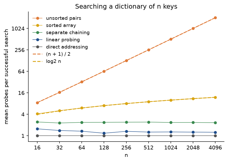
The same example measures the abstract data type's implementations side by side. At n = 4096 a successful search cost 2048.5 probes in an unsorted list of pairs, 12.0005 in a sorted array, 2.3293 in a chained table, 1.2542 in a linear-probing table at its default maximum load of one half, and 1 in a direct-address table over a universe of 65536 keys, which needed 65536 slots for 4096 keys.

When to use which

• Use dict and set for nearly everything in Python: they are hash tables with excellent constants, insertion order, and protection against flooding.
• Use collections.Counter for counting and collections.defaultdict for grouping; both are dicts.
• Use a sorted structure, such as a balanced search tree, bisect on a sorted list, or sortedcontainers, when you need order: minimum, maximum, successor, ranges or sorted iteration, or a guaranteed worst case.
• Use a direct-address table, a plain list indexed by the key, when the keys are small dense integers.
• Write your own table only to learn, or to control the layout: open addressing with linear probing for speed at moderate load and with a mixing hash, chaining when the load is unpredictable or entries must not move, double hashing or quadratic probing when the table must run nearly full.
• Use a trie when you need prefix queries, and a probabilistic structure when an approximate answer in much less memory will do.

Elsewhere

Java's HashMap chains entries in buckets of a power-of-two table, spreads the hash code by mixing its high bits into the low ones before taking the low bits, grows at a load of 0.75 and converts a bucket whose list grows long into a red-black tree, so a flood of colliding keys costs O(log n) per operation instead of O(n). C++'s std::unordered_map also chains, with a default maximum load of 1. Abseil's flat_hash_map, Rust's HashMap and, since version 1.24, Go's maps are Swiss tables: open addressing that probes whole groups of 8 or 16 slots at a time, moving from group to group by triangular steps like the ones above, with one metadata byte per slot holding seven bits of the hash so that a whole group is checked at once with vector instructions. Databases use hash tables for hash joins and in-memory indexes, compilers for their symbol tables, and caches pair one with a linked list to evict the least recently used entry, a combination Linked lists builds. The polynomial hash of this page reappears as the rolling hash of Rabin-Karp string matching, and memoization in dynamic programming is a dictionary from subproblems to answers.

Pitfalls

• Deleting from open addressing by emptying the slot. Every key placed beyond it on some probe path becomes unreachable, because searches stop at the first empty slot. In the worked example, emptying slot 1 loses 25, 50 and 63. Use a tombstone, or backward-shift deletion for linear probing; examples/common_mistakes.py runs this and every following mistake.
• Stopping a search at a tombstone. A tombstone means "keep going"; only an empty slot proves a key absent. Treating a tombstone as empty reports 25 missing after 38 is deleted.
• Inserting into the first tombstone without searching on. The key may already sit further along its path, and placing it at the first tombstone stores it twice: reinserting 63 after deleting 38 gives a table in which 63 appears twice. Search to an empty slot first, then use the first tombstone passed.
• Using quadratic probing without its guarantee. With h + i² and a table of 16 slots, five keys with home 3 fail at the fifth with 12 of 16 slots free; in a prime table of 7 slots, the fifth key with a shared home fails with 3 free. Use a prime size with the table at most half full, or a power-of-two size with triangular numbers. When tracing by hand, reduce every probe modulo m and check that the slot was not already tried.
• A second hash that can be zero or shares a factor with m. With h2(k) = k mod 7, the key 14 gets step 0 and probes its home slot forever; a step of 4 in a table of 12 slots visits only 3 of them. Use h2(k) = 1 + (k mod m′) with m′ < m and a prime m, or an odd step with a power-of-two m.
• Forgetting to wrap around. Probe sequences continue from slot m − 1 to slot 0; in the worked example 38 lands in slot 1 after trying 12 and 0. Reduce h(k) + offset modulo m at every probe, not just the home slot.
• A power-of-two size with the division method. k mod 2^p keeps only the low p bits, and keys that agree there collide: 1004 multiples of 32 used 8 of 256 buckets. Use a prime size, or mix the code with the multiplication method before taking low bits.
• Hashing strings by adding their characters. Anagrams such as spare, pears, reaps and parse collide in every table, and short words crowd into a narrow range of sums. Weight characters by position, as the polynomial hash does, with a base that shares no factor with the modulus.
• A hash code that keeps similar keys close. The polynomial hash puts words that differ in their last letter in neighbouring slots, which linear probing turns into long runs: 77.1584 probes per missing word at load 0.9 against the predicted 50.5015. Mix the code before reducing it when using linear probing.
• The multiplication method in floating point for large keys. Once k · A passes 2^53 the fractional part is gone, and a thousand keys near 10^17 all landed in one slot. Compute it in integers.
• Resizing without rehashing. A key's home k mod m changes with m, so the entries must be reinserted into the new array, not copied to the same index; copying lost all seven keys of the worked example.
• Growing by a fixed number of slots, or shrinking at half the maximum load. The first makes resizing cost Θ(n) per insertion on average (281.6388 moves per key at n = 20000 for steps of 64 slots, against 1.2837 for doubling); the second makes a table rebuild on every operation near the boundary.
• Letting tombstones pile up. A table that never rebuilds fills with tombstones until every missing-key search walks the whole array. Count keys plus tombstones against the maximum load and rebuild when they exceed it.
• Changing a key after inserting it, or defining equality without a matching hash. A key whose fields change is searched for in the wrong bucket and is found under neither its old nor its new value, in our tables and in dict alike; two equal objects with different hash codes both end up in a set.
• Expecting O(1) in the worst case or any order. Constant time is an expectation under well-spread keys, and iteration order says nothing about the keys; use a search tree when either matters.

Further reading

• D. E. Knuth, The Art of Computer Programming, volume 3, Sorting and Searching, second edition, section 6.4, Addison-Wesley, 1998. Hash functions, chaining, open addressing, the exact analysis of linear probing, deletion without tombstones (Algorithm R) and the estimates for secondary clustering.
• D. E. Knuth, "Notes on 'open' addressing", unpublished memorandum, 1963. The first analysis of linear probing.
• W. W. Peterson, "Addressing for random-access storage", IBM Journal of Research and Development 1(2), 130-146, 1957. Open addressing and its first measurements.
• T. H. Cormen, C. E. Leiserson, R. L. Rivest and C. Stein, Introduction to Algorithms, fourth edition, chapter 11, MIT Press, 2022. Chaining and open addressing under uniform hashing.
• R. Sedgewick and K. Wayne, Algorithms, fourth edition, section 3.4, Addison-Wesley, 2011. Separate chaining and linear probing in practice.
• L. J. Guibas and E. Szemerédi, "The analysis of double hashing", Journal of Computer and System Sciences 16(2), 226-274, 1978, and G. S. Lueker and M. Molodowitch, "More analysis of double hashing", Combinatorica 13(1), 83-96, 1993. Double hashing performs like uniform hashing.
• P. Flajolet, P. Poblete and A. Viola, "On the analysis of linear probing hashing", Algorithmica 22(4), 490-515, 1998. Linear probing, parking problems and the distribution of costs.
• A. Pagh, R. Pagh and M. Ružić, "Linear probing with constant independence", SIAM Journal on Computing 39(3), 1107-1120, 2009, and M. Pătraşcu and M. Thorup, "On the k-independence required by linear probing and minwise independence", ICALP 2010. Why linear probing needs better hash functions than chaining.
• The Python documentation of dict, set, object.__hash__ and the glossary entry "hashable", which state the rules for keys.