Quicksort¶

Quicksort puts n keys in order by choosing one key, the pivot, and splitting the others in a single pass into the keys that belong before it and the keys that belong after it; the pivot is then where it will stay, and the two sides are sorted the same way, independently. It sorts in place, its inner loop is a few instructions long, and on random input it makes about 2n ln n ≈ 1.39 n log2 n comparisons on average, which is why most standard libraries built their general-purpose sort on it for decades and why many still do. It also has a quadratic worst case, a recursion that can nest as deeply as the input is long, and an instability that surprises people who sort records. This page derives the two classic partitions, Lomuto's and Hoare's, with their loop invariants and traces, proves the recursion correct, compares pivot rules, derives the expected 2n ln n comparisons with indicator variables and checks it against counts, handles equal keys with three-way partitioning, bounds the stack at O(log n) by recursing on the smaller part, adds an insertion-sort cutoff and the introsort fallback to heapsort, and builds McIlroy's adversary that makes any deterministic pivot rule quadratic. Afterwards you will be able to trace any partition by hand, predict how a given variant behaves on sorted, reversed, repetitive and hostile input, and choose between your own quicksort, introsort and Python's sorted. It builds on Elementary sorts, uses the recurrences of Recurrences and the master theorem and the indicator variables of Counting and probability for algorithms, and is the natural companion of Merge sort.

The sorts need only the standard library; to run the plots, the notebook and the sample project install the base group, and the dev group for the tests.

Intuition¶

Picture a stack of a few hundred invoices to be put in order of amount. Take one invoice from the stack, say one for 340, and go through the rest once, laying every smaller amount on a pile to the left and every larger one on a pile to the right. Two things are now true that were not true before. The 340 invoice sits exactly where it belongs in the final order, because everything to its left is smaller and everything to its right is larger. And no invoice will ever have to cross it again: the left pile can be sorted without looking at the right pile, and the other way round. Do the same with each pile, then with each of their piles, and when every pile holds at most one invoice the whole stack is in order. There is nothing left to merge at the end.

The cost of one round is one look at every invoice, so the total cost depends on how many rounds deep the piles go. If the chosen invoice is near the middle of the amounts, each round halves the piles and about log2 n rounds suffice. If it is the smallest amount every time, one pile is always empty, the other shrinks by one, and the method makes about n²/2 comparisons, no better than the elementary sorts. Everything that follows is about making the good case likely and the bad case rare: choosing the pivot well, splitting equal amounts fairly, and keeping the bookkeeping of the piles small.

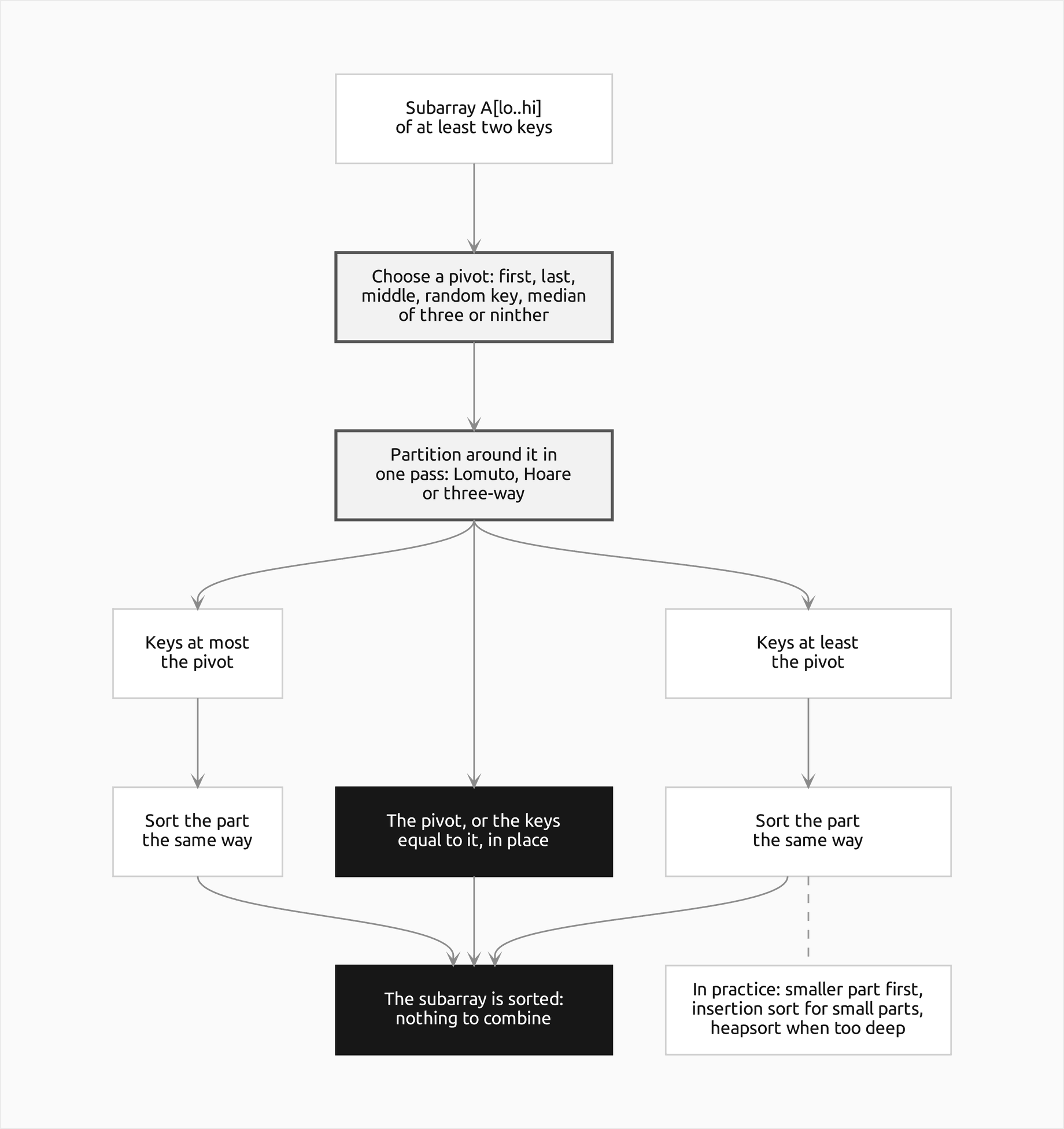
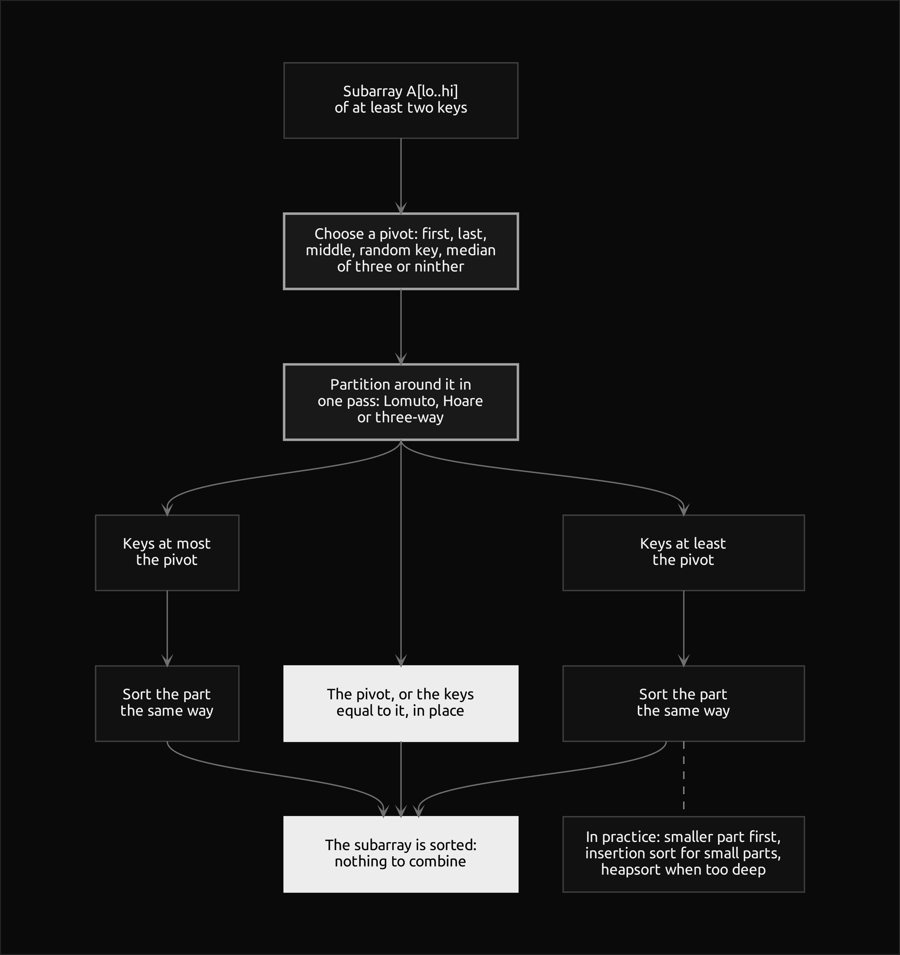
The diagram is the whole algorithm. The two outlined steps do all the work; the filled boxes are what is finished, the pivot after one partition and the whole subarray at the end; the note on the dashed line names the three engineering measures that turn the textbook algorithm into the one libraries ship.

How it works¶

Partition, then recurse¶

The sorting problem: given an array A of n keys that can be compared with less-than, rearrange it so that A[0] ≤ A[1] ≤ ... ≤ A[n − 1]. Quicksort works on a subarray A[lo..hi] and has three steps.

Choose a pivot x among the keys of A[lo..hi].
Partition: rearrange A[lo..hi] so that the keys at most x come first and the keys at least x come last. In the schemes that place the pivot, the result is an index q with the pivot in A[q] and this postcondition:

For lo at most k less than q, A of k is at most x; A of q equals x; for q less than k at most hi, A of k is at least x

Sort A[lo..q − 1] and A[q + 1..hi] recursively. A subarray of zero or one key is sorted already.

This is divide and conquer with the work at the front: dividing is the partition, conquering is the two recursive calls, and combining is free, because two sorted parts with every key of the first at most every key of the second are already a sorted whole. Merge sort is the mirror image: it divides blindly at the middle and does all the work in the merge. Quicksort needs no second array; apart from the recursion it sorts in place.

Partitioning is where the variants differ. There are three schemes in common use, each built around a loop invariant that says which part of the subarray is already classified:

Each bar shows the subarray in the middle of a partition. The region not examined shrinks by at least one key per step, and every other region grows only with keys that satisfy its promise. When no key is left to examine the partition is done, and the regions are the parts.

Lomuto's partition¶

Lomuto's scheme reads the pivot from the last slot, x = A[hi]. One index, j, walks from lo to hi − 1 and looks at each key once. A second index, i, marks the end of the keys known to be at most x, and starts at lo − 1 because that region is empty. The loop keeps this invariant before every test of A[j]:

For lo at most k at most i, A of k is at most x; for i less than k less than j, A of k is greater than x; A of hi equals x

Initially i = lo − 1 and j = lo, so both regions are empty and the invariant holds trivially. To maintain it, the loop tests A[j] ≤ x. If the test fails, A[j] simply joins the region of larger keys, which now ends at j. If it succeeds, i moves one slot right and A[i] and A[j] are exchanged: the slot i + 1 held the first larger key (or A[j] itself when no larger key has been seen), so the exchange puts the small key at the end of the small region and the larger key at the end of the large region. When j reaches hi, every key except the pivot is classified, and one last exchange of A[i + 1] with A[hi] puts the pivot between the two regions. It returns q = i + 1, and the postcondition holds with keys greater than x on the right.

The code is the loop above with a counter and a trace attached:

pivot = array[hi]
i = lo - 1
for j in range(lo, hi):
    key = array[j]
    small = not less(pivot, key, counter)
    record(trace, "lomuto-compare", (j,), (key, pivot), array, lo, hi, (("i", i), ("j", j)), small)
    if small:
        i += 1
        swap(array, i, j, counter, trace, lo, hi, (("i", i), ("j", j)))
place = i + 1
swap(array, place, hi, counter, trace, lo, hi, (("i", i), ("j", hi)), "place")

The test A[j] ≤ x is asked as "not x < A[j]", so every sort in the package compares keys with less-than only. Lomuto's scheme makes exactly m − 1 comparisons on a subarray of m keys, and one swap for every key at most the pivot plus one for the pivot itself. Some of those swaps exchange a slot with itself, while no larger key has been seen yet; the textbook code performs them anyway, and the counts here include them.

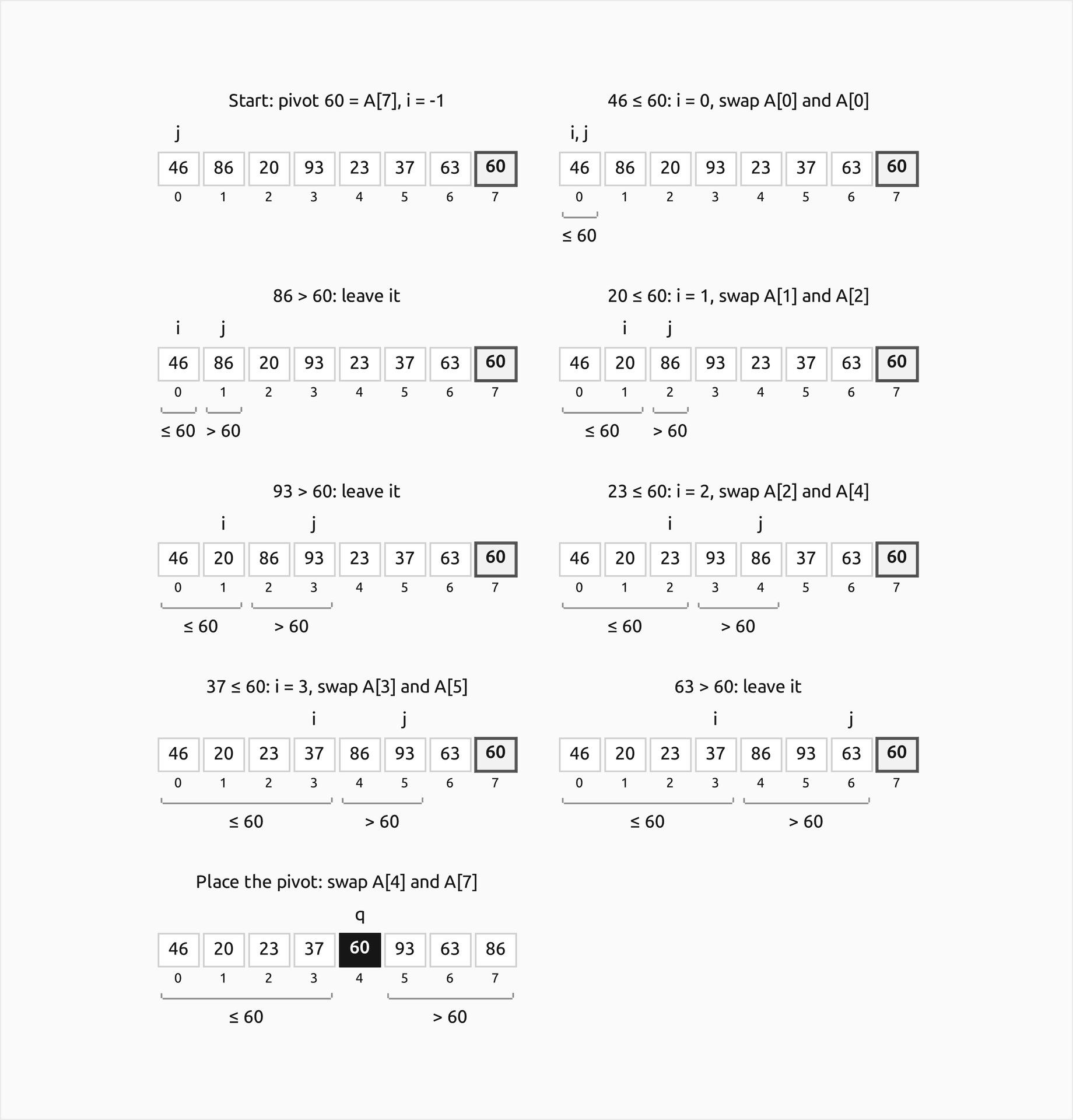
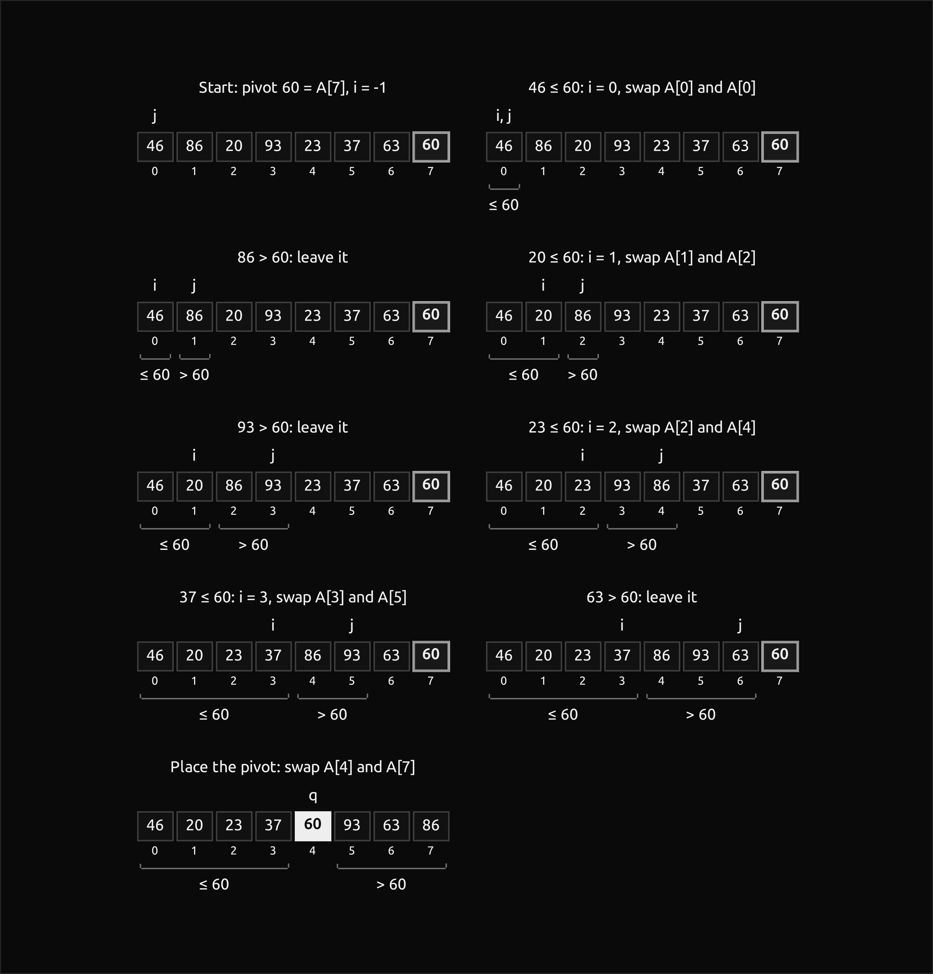
Nine states of Lomuto's partition of 46, 86, 20, 93, 23, 37, 63, 60 around the last key 60, two to a row and read left to right: brackets under the cells mark the keys at most 60 and the keys greater than 60, cells without a bracket are not yet examined, the pivot's cell is outlined, and i and j stand above their slots; the final state is 46, 20, 23, 37, 60, 93, 63, 86 with 60 filled at index 4 Nine states of Lomuto's partition of 46, 86, 20, 93, 23, 37, 63, 60 around the last key 60, two to a row and read left to right: brackets under the cells mark the keys at most 60 and the keys greater than 60, cells without a bracket are not yet examined, the pivot's cell is outlined, and i and j stand above their slots; the final state is 46, 20, 23, 37, 60, 93, 63, 86 with 60 filled at index 4

Each state is the array after one key has been examined, with the regions of the invariant bracketed underneath. The region at most 60 grows only when such a key arrives, by a swap with the first key greater than 60; the region greater than 60 grows by itself. The last state places the pivot, filled, at index 4, its final position.

Hoare's partition¶

Hoare's original scheme reads the pivot from the first slot, x = A[lo], and runs two scans towards each other. The left index i moves right until it finds a key at least x; the right index j moves left until it finds a key at most x. Both keys are on the wrong side, so they are exchanged, and the scans continue from there. When the indices meet or cross, j is returned. The invariant after every exchange is:

For lo at most k at most i, A of k is at most x; for j at most k at most hi, A of k is at least x; and on return, lo is at most j which is less than hi

Three details make the scheme correct. First, the scans never run off the subarray. On the first round the left scan stops at once, at the pivot itself in A[lo], and the right scan stops at A[lo] at the latest. On every later round each scan stops at the latest at the key the previous exchange put on its far side: the right scan cannot pass the small key now at i, and the left scan cannot pass the large key now at j. Second, both scans stop on keys equal to the pivot. That costs exchanges between equal keys, but it is exactly what keeps a run of equal keys from being split all to one side. Third, the returned j satisfies lo ≤ j < hi, so both parts A[lo..j] and A[j + 1..hi] are nonempty and strictly smaller than the subarray, and the recursion makes progress.

The price of this economy is that the pivot does not end in its final position. It is somewhere in one of the two parts, and the recursion must include it: the parts are A[lo..j] and A[j + 1..hi], not A[lo..j − 1] and A[j + 1..hi]. Mixing up the two return conventions is the most common bug in quicksort code, and it produces either a wrong order or a recursion that never ends; the pitfalls section shows both.

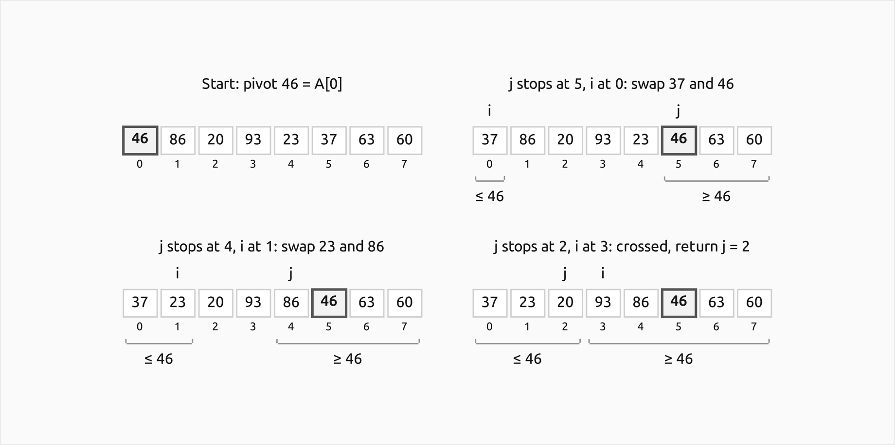
The bracketed keys on the left are known to be at most 46 and those on the right at least 46. Only two exchanges were needed, against five for Lomuto on the same keys, and the pivot, outlined, ended at index 5, inside the right part, while its sorted position is 3.

Many textbooks and libraries use a variant that keeps the two scans but places the pivot: it leaves the pivot in A[lo] while the scans run over A[lo + 1..hi], then exchanges it with A[j], the last key of the left region. The left scan must then check that it has not reached hi, because nothing to its right is guaranteed to stop it. This variant returns a final pivot position q, like Lomuto's, and the package calls it hoare_placed_partition.

Lomuto and Hoare compared¶

The two schemes solve the same problem with different trade-offs:

Where the pivot ends. Lomuto's scheme and the placed variant put the pivot at its final index and leave it out of both parts. Hoare's original scheme returns a boundary, not a position, and the pivot stays inside a part.
Comparisons per partition. Lomuto's scheme makes exactly m − 1 on m keys; Hoare's scans compare each key about once, plus one or two extra tests where they cross:

Lomuto makes m minus 1 comparisons on m keys, Hoare m plus 1 or m plus 2; three-way partitioning makes between m minus 1 and 2 times m minus 1

Swaps. Lomuto swaps every key at most the pivot, about half the keys, whether it is misplaced or not. Hoare swaps only pairs that are both on the wrong side, about a sixth of the keys on random input. Over a whole sort of random keys that is about n ln n swaps for Lomuto against about a third of that for Hoare, as the cost section measures.
Equal keys. Lomuto sends every key equal to the pivot to the left, so an array of equal keys splits n − 1 against 0 every time and the sort becomes quadratic. Hoare's scans stop on equal keys and meet in the middle, so equal keys split evenly.
Simplicity. Lomuto's loop is easier to get right and to prove, which is why it is the usual first presentation; Hoare's is faster and more robust, which is why production code descends from it.

The recursion and why it is correct¶

The sort is the partition applied recursively. The body of quicksort_recursive in recursive.py:

hi = len(array) - 1 if hi is None else hi
if hi <= lo:
    return array
gauge.enter()
record(trace, "call", (lo, hi), (), array, lo, hi, detail=gauge.current)
left, right = partition_step(array, lo, hi, scheme, pivot, counter, rng, trace)
quicksort_recursive(array, *left, scheme, pivot, counter, gauge, trace, rng)
quicksort_recursive(array, *right, scheme, pivot, counter, gauge, trace, rng)
gauge.leave()
return array

partition_step chooses the pivot by the rule, moves it into the slot the scheme reads it from, partitions, and returns the two ranges still to sort; the gauge records how deep the calls nest.

Correctness is an induction on the length m = hi − lo + 1. A subarray with m ≤ 1 is sorted. For m ≥ 2, the partition leaves every key of the left part at most every key of the right part, with the pivot (when it is placed) between them. Both parts are shorter than m: with a placed pivot because the pivot is excluded, and with Hoare's boundary because both parts are nonempty. By the induction hypothesis the recursive calls sort both parts, and they rearrange keys only within their own part, so the order between the parts survives. A sorted left part followed by the pivot and a sorted right part, with no key of the left exceeding any key of the right, is sorted. The same induction proves termination, since every call works on a strictly shorter subarray.

The calls form a binary tree, the recursion tree, and drawing it is the best way to trace a whole sort by hand:

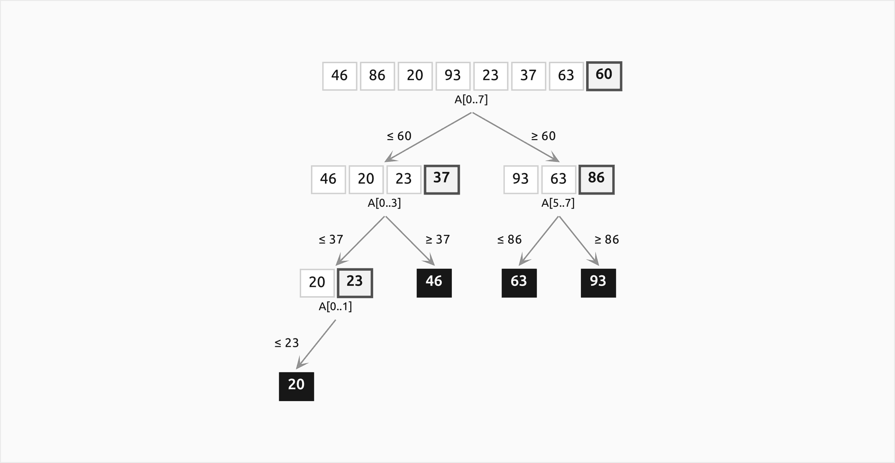
Each node is the subarray a call receives, with its pivot outlined and its range underneath; the filled leaves are single keys, already in place. The tree has depth 3 and four internal nodes, one partition each. Its shape decides the cost: the comparisons of a level are at most the number of keys on it, so a short, bushy tree is cheap and a tall, thin one is expensive.

Choosing the pivot¶

Every scheme reads its pivot from a fixed slot, the last for Lomuto and the first for the others. A pivot rule picks an index, and the package swaps that key into the slot before partitioning, so any rule works with any scheme. The rules:

First or last key. No work at all, and fine on random input, but a sorted or reverse-sorted input makes every pivot the smallest or the largest key of its subarray. One part is then empty, the other shrinks by one, and the sort makes n(n − 1)/2 comparisons, the worst case. Sorted and nearly sorted inputs are common in practice, which rules these out for library code.
Middle key. Perfect on sorted and reversed input, but some simple patterns, such as the organ pipe that rises and falls, defeat it.
Random key. The expected cost is the same for every input, about 1.39 n log2 n comparisons, because the randomness is in the algorithm, not in the data. Bad runs remain possible but are astronomically unlikely, as the cost section shows.
Median of three. The median of the first, middle and last keys. On sorted input it picks the true median and splits perfectly; on random input it lowers the expected comparisons to about 1.19 n log2 n, because the median of three is more likely than a single key to land near the middle. The package orders the three samples in place, so that the smallest ends first and the largest last, and then uses the middle one. Ordering them matters: finding the median without moving the samples interacts badly with the placed Hoare partition and turns reversed input quadratic, a trap the pitfalls section measures.
Ninther. Tukey's median of three medians of three, spread across the subarray: up to twelve comparisons to get a pivot much closer to the true median, worth it only on large subarrays. Libraries use it above a size threshold.

Deterministic rules have one more weakness, McIlroy's adversary, which constructs a bad input for any of them; it has its own section below.

Equal keys and three-way partitioning¶

When many keys are equal, two-way partitioning wastes work: keys equal to the pivot go into the parts and are partitioned again and again, although they are already in their final relative place. Three-way partitioning, after Dijkstra's Dutch national flag problem, splits the subarray into keys less than, equal to and greater than the pivot in one pass, and recurses only on the outer two. It keeps three indices: lt, the end of the less region, i, the next key to examine, and gt, the start of the greater region. The invariant before every examination:

For lo at most k less than lt, A of k is less than x; for lt at most k less than i, A of k equals x; A of k is unexamined for i at most k at most gt; for gt less than k at most hi, A of k is greater than x

A key less than x is swapped with the first equal key at lt, and both lt and i advance. A key greater than x is swapped with the last unexamined key at gt, and gt retreats, but i stays: the key that came back from gt has not been examined yet. A key equal to x only advances i. Each step shrinks the region not examined by one, and each key costs one comparison if it is less than x and two otherwise.

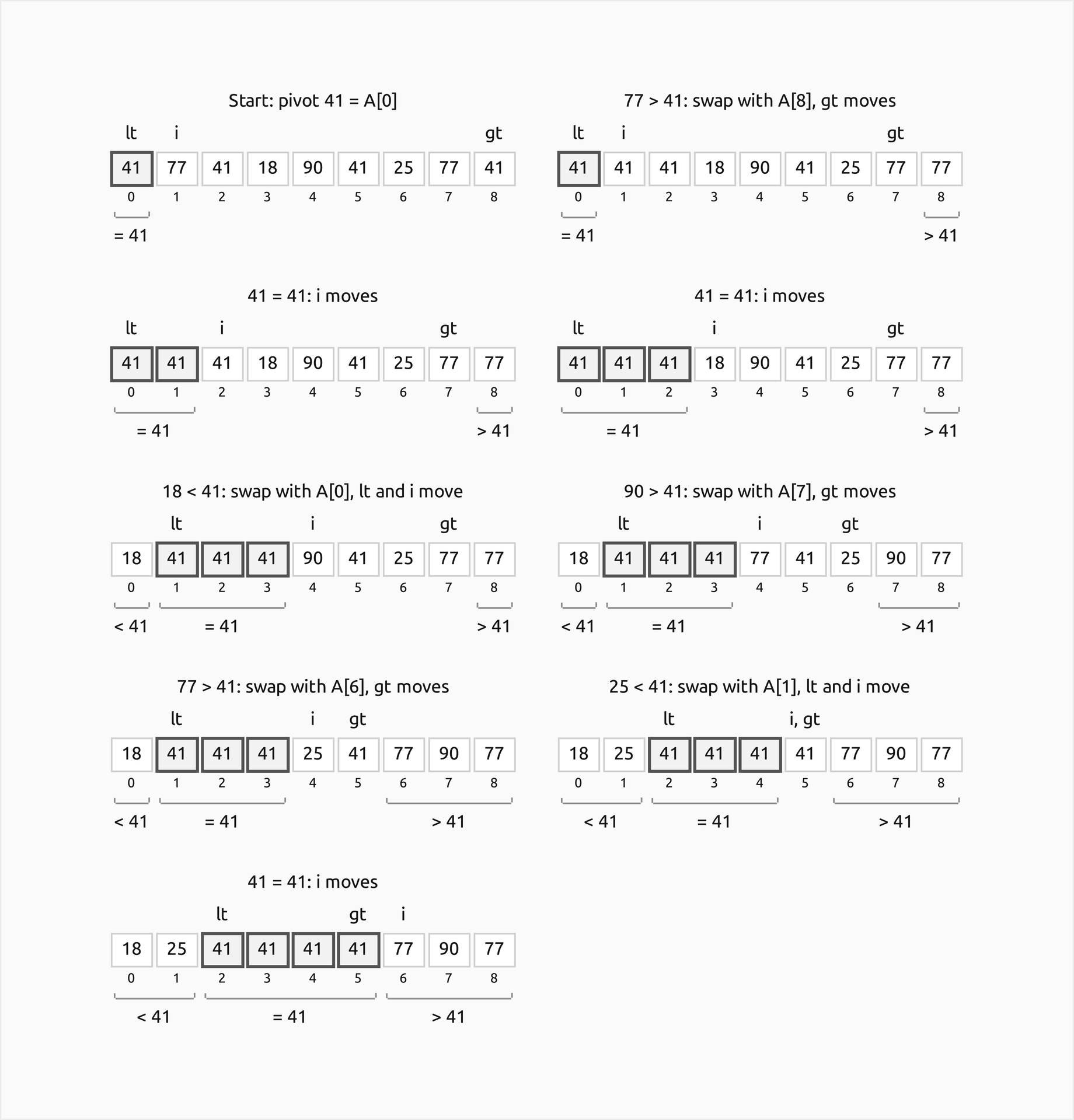
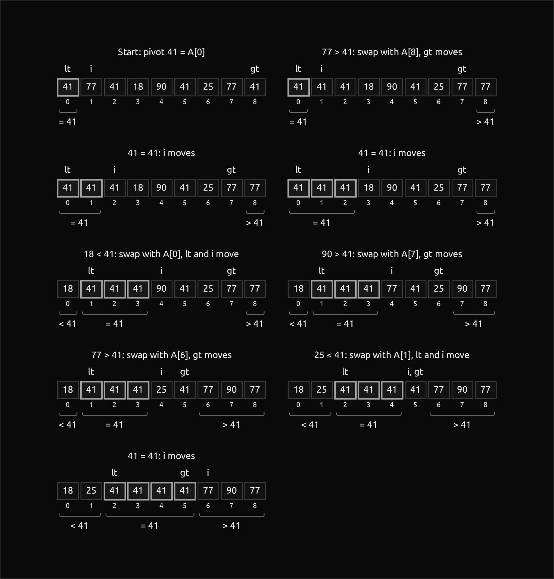
The outlined block of keys equal to 41 grows in the middle and is finished when the pass ends. Note the second state: the 41 that arrives from the end is examined next, because i did not move, and the same happens to the 77 and the 25 further down. On an array of n equal keys the whole sort is a single pass of 2(n − 1) comparisons.

Recursion depth and the smaller part first¶

Quicksort's only extra memory is the recursion stack, and its depth is the height of the recursion tree. With balanced splits that is about log2 n, but on sorted input with a fixed end pivot every call has one empty part and the calls nest n − 1 deep. Python's default recursion limit is about 1000 frames, so the textbook recursion fails on a sorted list of a few thousand keys long before it would finish its quadratic work; in C it overflows the stack. Removing the second recursive call by looping, which a compiler does for a tail call, does not help by itself: if the part left to the call is the large one, the nesting is just as deep.

The fix is to recurse on the smaller part and loop on the larger one:

while lo < hi:
    record(trace, "call", (lo, hi), (), array, lo, hi, detail=gauge.current)
    left, right = partition_step(array, lo, hi, scheme, pivot, counter, rng, trace)
    if size(left) <= size(right):
        quicksort_smaller_first(array, *left, scheme, pivot, counter, gauge, trace, rng)
        lo, hi = right
    else:
        quicksort_smaller_first(array, *right, scheme, pivot, counter, gauge, trace, rng)
        lo, hi = left

A part handed to a nested call holds at most (m − 1)/2 keys of a range of m, so the sizes along any chain of nested calls more than halve. If the deepest nested call that partitions has s_d ≥ 2 keys, the one above it had at least 2s_d + 1 ≥ 5, the one above that at least 11, and the outermost at least 3 · 2^(d − 1) − 1:

If each nested size s k plus 1 is at most s k minus 1 over 2, then s k is at least 2 s k plus 1 plus 1; with s d at least 2 this gives n at least 3 times 2 to the d minus 1, minus 1; so d is at most the floor of log2 of n plus 1 over 3, plus 1, which is at most log2 n

So the stack never holds more than about log2 n frames, on every input, sorted, random or adversarial, while the comparisons and swaps are exactly those of the plain recursion. The package's engine.quicksort runs every variant on an explicit stack instead of Python's, so that measurements never hit the recursion limit, and reports the depth the recursive program would reach: two calls per partition (left-first), the tail call looped (tail-loop), or the smaller part first (smaller-first).

Small parts: an insertion-sort cutoff¶

Near the leaves of the recursion tree quicksort spends its time on tiny subarrays, where choosing a pivot, partitioning and calling again cost more than they save. Insertion sort, which makes few comparisons on a handful of keys and has no overhead at all, does better there. The cutoff M hands every part of at most M keys to insertion sort. Its average cost on m keys in random order is:

The expected comparisons of insertion sort on m keys are m times m minus 1 over 4, plus m, minus H m

For a handful of keys that is comparable to quicksort's own count, 72.6 against 50.9 expected comparisons at m = 16, so the cutoff changes the total comparisons only a little while removing most of the calls: with a random pivot about 2n/(M + 2) partitions remain instead of 2n/3, about (M + 2)/3 times fewer. Libraries choose M between about 10 and 30 by timing on their own machines; the cost section shows the trade-off in counts.

Introsort¶

Randomization makes the quadratic case unlikely; introsort, Musser's introspective sort, makes it impossible. It runs quicksort with a median-of-three pivot and watches the depth of every path: once a path has partitioned more than 2⌊log2 n⌋ times, which never happens with reasonable splits, it stops partitioning that subarray and sorts it with heapsort, whose worst case is O(m log m). Parts of at most 16 keys go to insertion sort, and the smaller part is sorted first. The bound follows level by level:

The limit is 2 times the floor of log2 n partitioning levels on any path; the comparisons are at most 2 floor log2 n times c n for the partitioning levels, plus 2 n log2 n for heapsort, plus O of n, which is O of n log n

Each partitioning level costs at most about n comparisons, since the parts on one level are disjoint, there are at most 2⌊log2 n⌋ levels, and heapsort sorts whatever remains in at most about 2n log2 n comparisons, so the total is O(n log n) in the worst case, about 4n log2 n at most. On ordinary inputs the limit is never reached and introsort is simply a well-engineered quicksort. The package carries a small heapsort on a subarray in heapsort.py; the full treatment of heaps is in Heaps and priority queues, and a test checks that both heapsorts agree.

Quicksort is not stable¶

A sort is stable if keys that compare equal keep their input order. Quicksort is not, and no cheap change makes it so. Partitioning exchanges keys across long distances: Lomuto's scheme moves the first larger key it meets to wherever the next small key was, past any number of keys in between, and Hoare's exchanges pairs from opposite ends. Sorting the records 7a, 3a, 7b, 5a, 3b, 5b by their numbers alone, Lomuto's quicksort returns 3a, 3b, 5a, 5b, 7b, 7a: the two sevens have changed places. When stability matters, sort with a stable algorithm such as merge sort or Python's sorted, or make the keys unique by attaching the input position, sorting (key, position) pairs, which is what the package's stable_quicksort does.

McIlroy's adversary¶

Any deterministic pivot rule, however clever, has inputs that make it quadratic, and McIlroy showed how to construct them automatically for any implementation, without reading its code. The adversary plays the role of the keys. It runs the sort on stand-ins, called probes here, and answers each comparison on the fly, committing to actual values only when it must:

Every key starts as gas, a value larger than anything decided so far.
When two gas keys are compared, the adversary freezes one of them to the next solid value, smaller than all gas. It freezes the pivot candidate, the gas key most recently compared with a solid one, if that is one of the two.
Comparisons involving a solid key are answered by the values.

A quicksort compares its pivot with key after key, so the pivot becomes the candidate and is frozen to the smallest value still available. The partition then puts nearly everything on one side, and the same happens at the next level. When the sort finishes, the remaining gas keys are frozen in any order, which is consistent with every answer given. Sorting the resulting input again with the same deterministic algorithm asks exactly the same comparisons and gets the same answers, so it reproduces the quadratic run: against the median of three, about n²/4 comparisons.

The attack needs a deterministic algorithm. Against randomized quicksort it can only build an input for the particular random choices of one run; sorted again with another seed, that input is as easy as any other. That is why a randomized pivot defends against adversaries only if its seed is secret, and why introsort, which bounds the damage whatever the input, is the standard choice where untrusted data is sorted.

Cost¶

Every case at a glance¶

For n keys:

Worst case: Θ(n²) comparisons, n(n − 1)/2 exactly for Lomuto's scheme on sorted input with the last key as pivot, and a recursion depth of n − 1 unless the smaller part is handled first.
Best case: about n log2 n comparisons, when every pivot is the median of its subarray.
Expected, with a random pivot on any input, or with any fixed rule on random input: 2(n + 1)H(n) − 4n comparisons, about 1.39 n log2 n.
Median of three: about 1.19 n log2 n expected comparisons on random input; still Θ(n²) in the worst case.
Introsort: O(n log n) comparisons in the worst case.
Extra space: O(log n) for the stack when the smaller part is sorted first, otherwise up to n − 1 frames; no extra array.

The distinction between worst case and expected matters more here than for any other sort in this part. Merge sort and heapsort are O(n log n) on every input; quicksort is fast on average and slow on rare inputs, and whether those inputs are rare depends on who supplies them.

The worst case¶

When every partition leaves one part empty, the recursion peels off one key per level. With Lomuto's m − 1 comparisons per partition:

T of n equals T of n minus 1 plus T of 0 plus n minus 1, with T of 0 and T of 1 equal to 0; so T of n is n minus 1 plus n minus 2 and so on down to 1, the sum of k for k from 1 to n minus 1, which is n times n minus 1 over 2, Theta of n squared

Sorted input with the last key as pivot does exactly this, and so does reversed input: the first pivot is the smallest key, the partition puts the largest key at the end, and the rest is again reversed. The example worst_case_and_depth.py counts both and two remedies:

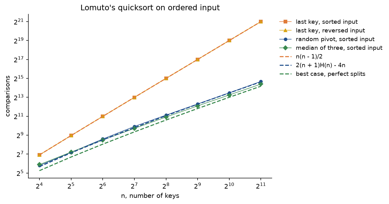
The last-key pivot on sorted keys makes exactly n(n − 1)/2 comparisons at every n, 2096128 for 2048 keys, and on reversed keys exactly the same number. A random pivot on the same sorted keys makes 26191.4 on average, 3 percent above the prediction of 25420.1, and the median of three makes 21514, close to the best case. A factor of 80 separates the same algorithm with two pivot rules at only 2048 keys.

The best case and balanced splits¶

If every pivot is the median, the m − 1 other keys split as evenly as possible:

B of n equals n minus 1 plus B of the floor of n minus 1 over 2 plus B of the ceiling of n minus 1 over 2; for n equal to 2 to the k minus 1, B equals k minus 2 times 2 to the k, plus 2, which is n plus 1 times log2 of n plus 1, minus 2n, Theta of n log n

The splits need not be even for the cost to be n log n. Any split in a fixed proportion keeps the recursion tree logarithmic, because the longest path shrinks the subarray by a constant factor at each step:

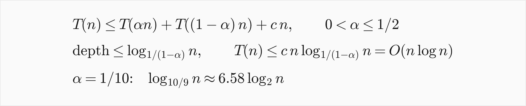
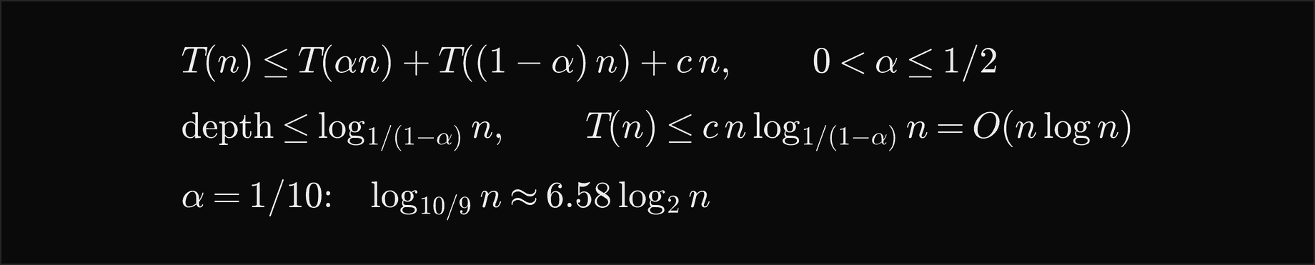
T of n is at most T of alpha n plus T of 1 minus alpha times n plus c n for alpha between 0 and one half; the depth is at most log base 1 over 1 minus alpha of n, so T of n is at most c n times that logarithm, O of n log n; for alpha equal to one tenth the depth is log base 10 over 9 of n, about 6.58 log2 n T of n is at most T of alpha n plus T of 1 minus alpha times n plus c n for alpha between 0 and one half; the depth is at most log base 1 over 1 minus alpha of n, so T of n is at most c n times that logarithm, O of n log n; for alpha equal to one tenth the depth is log base 10 over 9 of n, about 6.58 log2 n

Even a split of 1 to 9 at every level costs only a constant factor more than perfect halving. The danger is not unbalanced splits but splits that leave a constant number of keys on one side, level after level.

The expected number of comparisons¶

Take randomized quicksort with Lomuto's partition: each pivot is chosen uniformly from its subarray. Name the keys by rank, z_1 < z_2 < ... < z_n, and let X_ij be 1 if z_i and z_j are ever compared and 0 otherwise. Every comparison is between a pivot and another key of its subarray, and after the partition the pivot is excluded from both parts, so no pair is compared twice and the total count C is the sum of the indicators. Linearity of expectation turns the expected count into a sum of probabilities, with no independence needed:

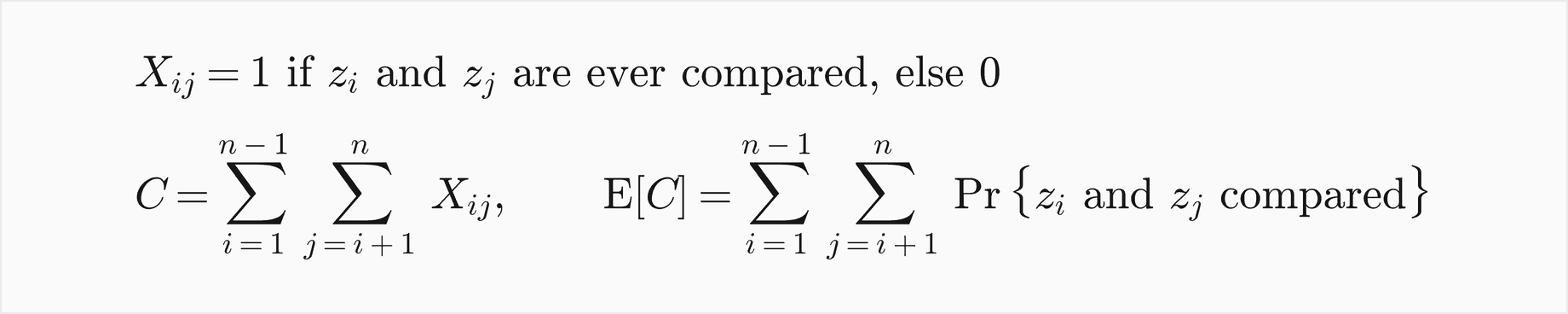
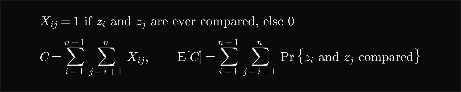
X i j is 1 if z i and z j are ever compared and 0 otherwise; C is the sum of X i j over all pairs i less than j, and the expected value of C is the sum over all pairs of the probability that z i and z j are compared

Now consider the keys z_i, z_(i+1), ..., z_j, a block of j − i + 1 consecutive ranks. As long as no pivot has been chosen from this block, all of its keys stay in the same subarray. The first pivot chosen from the block decides the pair: if it is z_i or z_j, that key is compared with every other key of its subarray, including the other one; if it is any key strictly between them, it sends z_i to one side and z_j to the other, and they are never compared. Since the pivot is uniform over its subarray, every key of the block is equally likely to be the first chosen:

The probability that z i and z j are compared equals the probability that the first pivot chosen from z i to z j is z i or z j, which is 2 over j minus i plus 1

Neighbours in rank are always compared, which is necessary since nothing else could tell them apart, and the smallest and largest keys are compared with probability only 2/n. Summing over the pairs, grouped by their rank distance d = j − i, of which there are n − d:

The expected value of C is the sum over d from 1 to n minus 1 of n minus d times 2 over d plus 1, which is the sum over k from 2 to n of n plus 1 minus k times 2 over k; that equals 2 times n plus 1 times H n minus 1, minus 2 times n minus 1, which is 2 times n plus 1 times H n, minus 4n

Here H(n) is the harmonic number, which grows like the natural logarithm:

H n is 1 plus one half plus and so on up to 1 over n, which equals ln n plus gamma plus O of 1 over n, with gamma equal to 0.5772

so the expectation is 2n ln n to leading order, which in base 2 is the famous constant 1.39:

2 times n plus 1 times H n minus 4n equals 2n ln n minus 4 minus 2 gamma times n plus O of log n, which is about 1.3863 n log2 n minus 2.8456 n

The same result comes from the recurrence of the average cost, conditioning on the rank q of the first pivot, which is uniform, and solving by the telescoping trick of multiplying by n and subtracting the equation for n − 1:

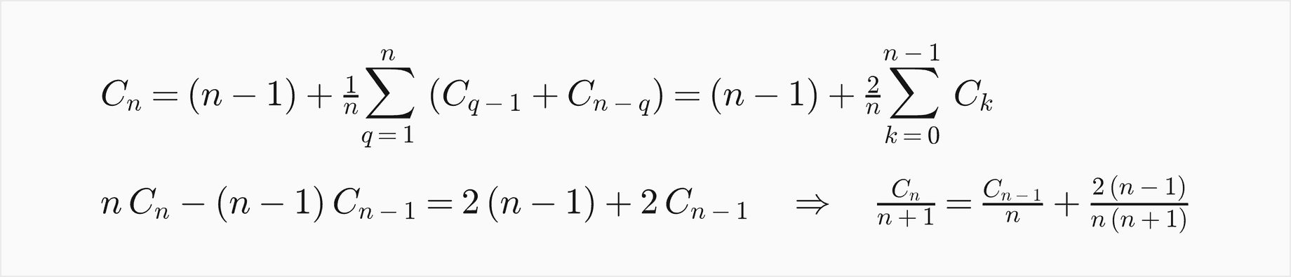
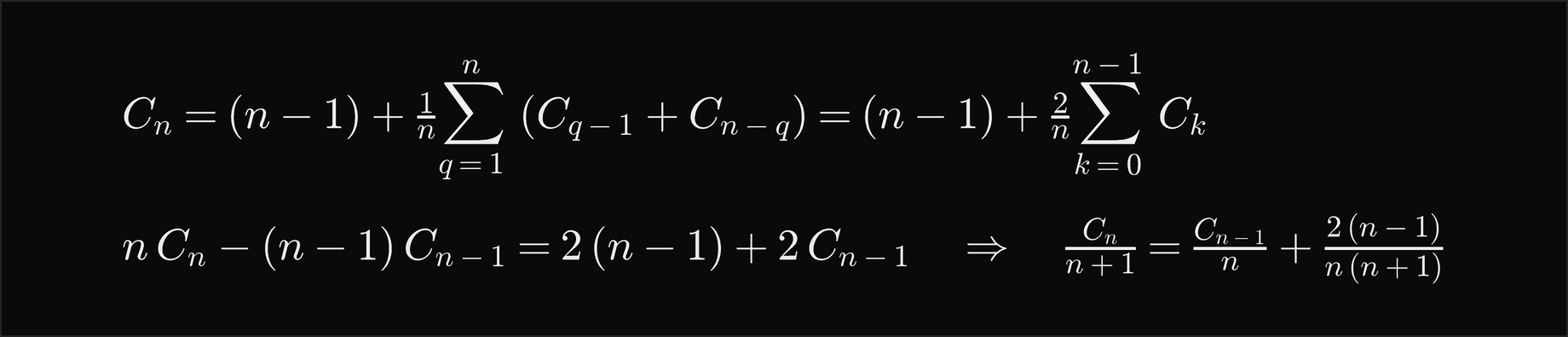
C n equals n minus 1 plus 1 over n times the sum over q from 1 to n of C q minus 1 plus C n minus q, which is n minus 1 plus 2 over n times the sum over k from 0 to n minus 1 of C k; then n C n minus n minus 1 times C n minus 1 equals 2 times n minus 1 plus 2 C n minus 1, so C n over n plus 1 equals C n minus 1 over n plus 2 times n minus 1 over n times n plus 1 C n equals n minus 1 plus 1 over n times the sum over q from 1 to n of C q minus 1 plus C n minus q, which is n minus 1 plus 2 over n times the sum over k from 0 to n minus 1 of C k; then n C n minus n minus 1 times C n minus 1 equals 2 times n minus 1 plus 2 C n minus 1, so C n over n plus 1 equals C n minus 1 over n plus 2 times n minus 1 over n times n plus 1

The indicator argument is shorter and explains where the cost comes from: from the pairs far apart in rank, which are rarely compared but are many. The tests check that the sum of indicators, the recurrence and the closed form agree, and the example expected_comparisons.py checks the pair probability itself by counting: over 20000 runs on 10 keys, the frequency with which each of the 45 pairs met differed from 2/(j − i + 1) by at most 0.0051, and no pair was ever compared twice. Two pitfalls hide in such an experiment. The input must not be generated from the same seeded generator as the pivots, or the two become correlated: with a shared seed, the smallest and largest keys met in 0.2934 of the runs instead of 0.2. And the expectation is over the algorithm's coins for a fixed input, so the example keeps the input fixed, sorted even, and varies only the pivot seed.

Counted over 12 random permutations for each n:

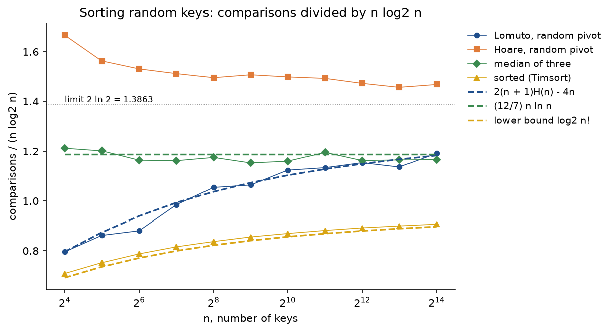
At n = 16384 Lomuto's randomized quicksort averaged 273320.4 comparisons against the predicted 271382.4, that is 1.1916 against 1.1831 n log2 n; the ratio climbs towards its limit 1.3863 only slowly, because the term −2.8456n is still large at these sizes. Hoare's original scheme makes more comparisons, 1.4676 n log2 n: its partitions test the crossing keys twice, and because the pivot stays inside a part it takes part in later partitions too, so the recursion always performs exactly n − 1 partitions. Its strength is elsewhere, in the swaps.

How concentrated the count is¶

An expected value is a promise about averages; the variance says how far a single run can stray. The exact variance of randomized quicksort's comparison count is known, and its square root grows only linearly:

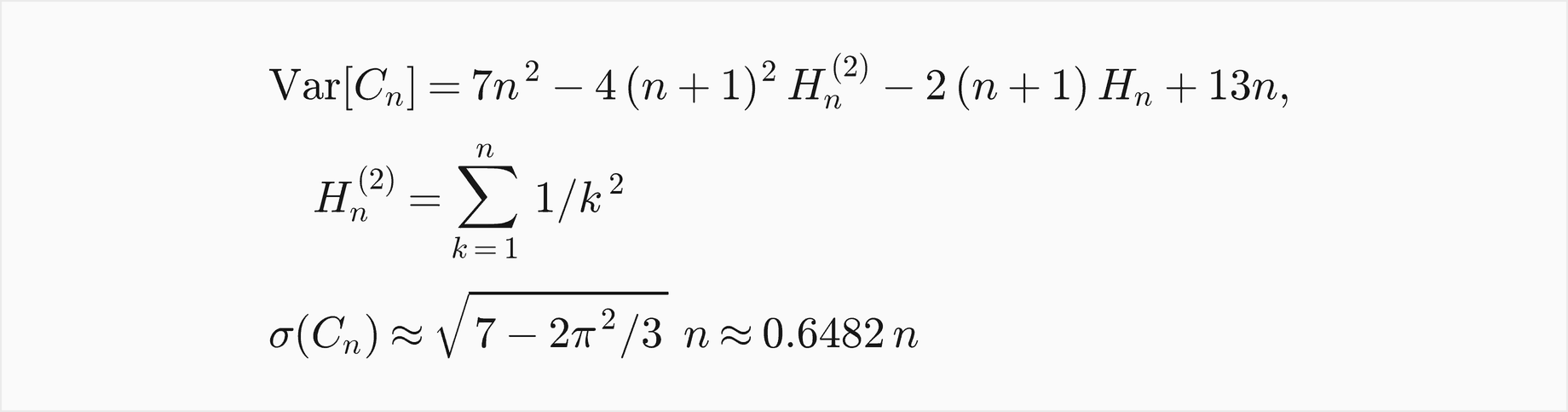
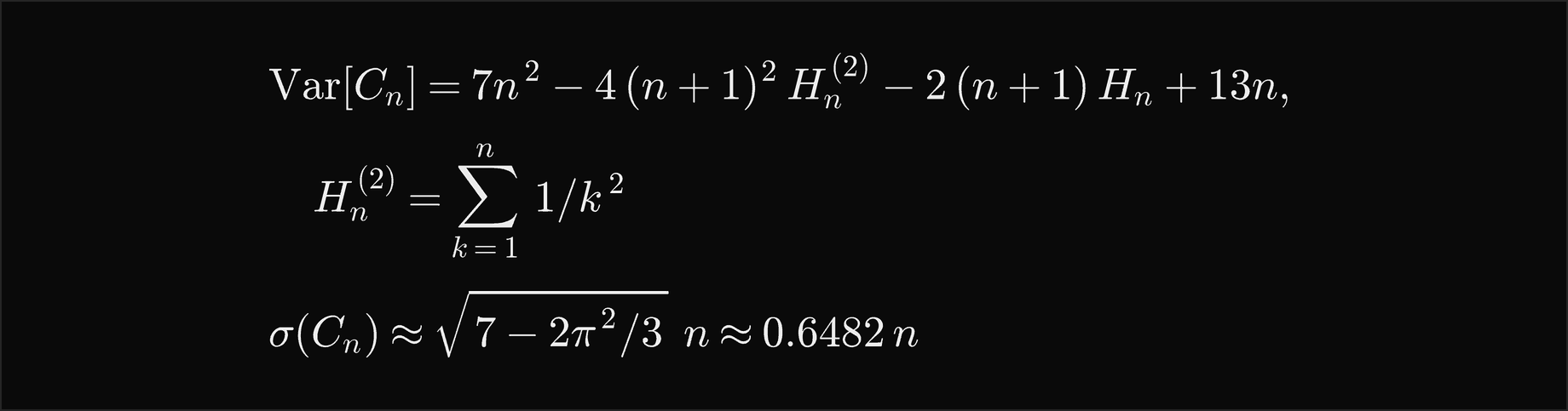
The variance of C n is 7 n squared minus 4 times n plus 1 squared times H n of order 2, minus 2 times n plus 1 times H n, plus 13 n, where H n of order 2 is the sum of 1 over k squared; the standard deviation is about the square root of 7 minus 2 pi squared over 3, times n, about 0.6482 n

The mean grows like n log n and the spread like n, so relative to the mean the spread shrinks like 1/log n: large runs are almost never far from average.

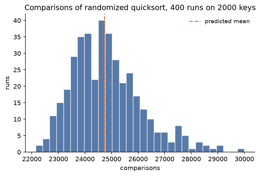
Histogram of the comparison counts of 400 runs of randomized quicksort on 2000 keys, between about 22000 and 30000, peaked near the dashed predicted mean of 24730 and with a longer tail to the right

The 400 runs averaged 24823.5 comparisons against the predicted 24729.8, with a standard deviation of 1323.8 against the predicted 1286.9, which is 0.6434 n at this size. The smallest run took 22149 and the largest 30005, while the worst case for 2000 keys is 1999000: not one run in 400 came within a factor of 60 of it. The distribution is skewed to the right, unlucky early pivots making the long tail, and its limit is not a normal distribution.

Swaps and partitions¶

The same recurrence with other tolls gives the other counts. Each Lomuto partition is one call, and with a pivot of rank r it swaps r times, (m + 1)/2 on average:

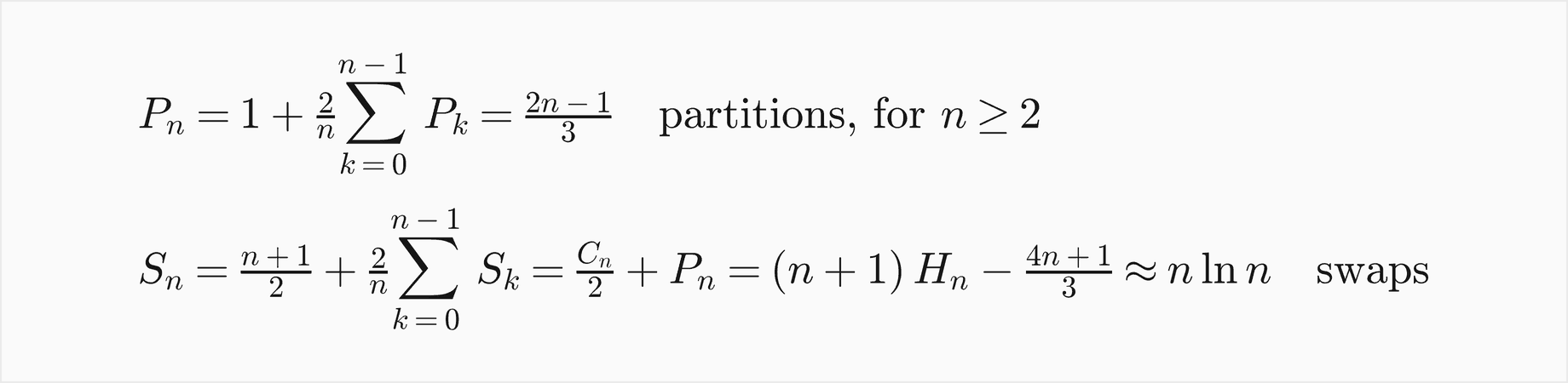
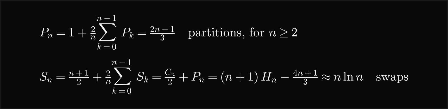
P n equals 1 plus 2 over n times the sum of P k, which solves to 2n minus 1 over 3 partitions for n at least 2; S n equals n plus 1 over 2 plus 2 over n times the sum of S k, which equals C n over 2 plus P n, that is n plus 1 times H n minus 4n plus 1 over 3, about n ln n swaps

Over 200 random permutations of 2000 keys, Lomuto's quicksort made 13642.1 swaps on average against the predicted 13697.9, which is 0.9011 n ln n, and 1333.2 partitions against (2n − 1)/3 = 1333.0. Hoare's scheme on the same inputs made 5146.5 swaps, 0.3385 n ln n, about a third of Lomuto's, in exactly 1999 partitions, and 34449.9 comparisons against Lomuto's 24762.8, 1.39 times as many. On machines where moving data is expensive and comparing is cheap, Hoare's trade wins, which is why it is the scheme production code descends from.

The median of three¶

With the median of three random keys as pivot, the pivot's rank is no longer uniform: rank k is the median when one sample is below it and one above it:

The probability that the pivot has rank k is k minus 1 times n minus k divided by n times n minus 1 times n minus 2 over 6, for 1 less than k less than n; the expected comparisons are about 12 over 7 n ln n, which is about 1.1883 n log2 n

Solving the recurrence with these probabilities replaces the constant 2 by 12/7. The package's median of three, ordering the first, middle and last keys and partitioning with the placed Hoare scheme, made 267562.8 comparisons at n = 16384, 1.1665 n log2 n, even though it pays three comparisons per partition for its samples. That is a little below the leading term, because, as with a single random pivot, the next term of the expansion is negative. On sorted and reversed input it splits perfectly. Its worst case is still quadratic.

Equal keys¶

On n equal keys the three schemes behave completely differently:

Lomuto makes n times n minus 1 over 2 comparisons on n equal keys; Hoare's scans meet in the middle, E of n equals n plus 2 plus 2 E of n over 2, about n log2 n; three-way partitioning makes 2 times n minus 1

The example equal_keys_and_adversary.py counts all three, and then varies the number of distinct values:

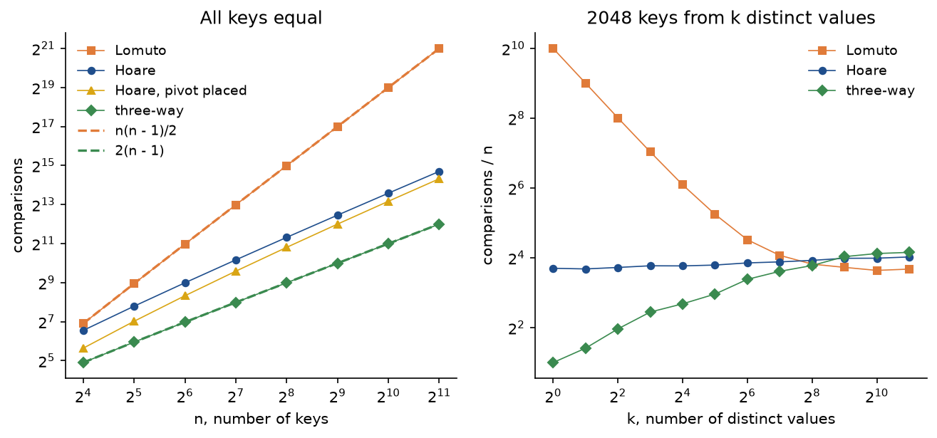
All counts match their formulas exactly: 2096128 comparisons for Lomuto on 2048 equal keys, 26622 for Hoare and 4094 for three-way partitioning. The right panel shows the trade-off. Three-way partitioning wins clearly while there are few distinct values, 5.45 comparisons per key against 13.66 for Hoare with 8 values, because each value is finished in the pass that meets it, so the cost grows with log k rather than log n. With all keys distinct it loses, 17.82 per key against 12.79 for Lomuto, because every key that is not less than the pivot pays a second comparison. Lomuto's scheme is unusable with many repeats, 1023.5 comparisons per key when all are equal. Libraries reconcile the two by partitioning two ways and switching to three ways only when they detect equal keys.

Recursion depth measured¶

The depth of the recursion depends on how it is organised, not only on the pivots:

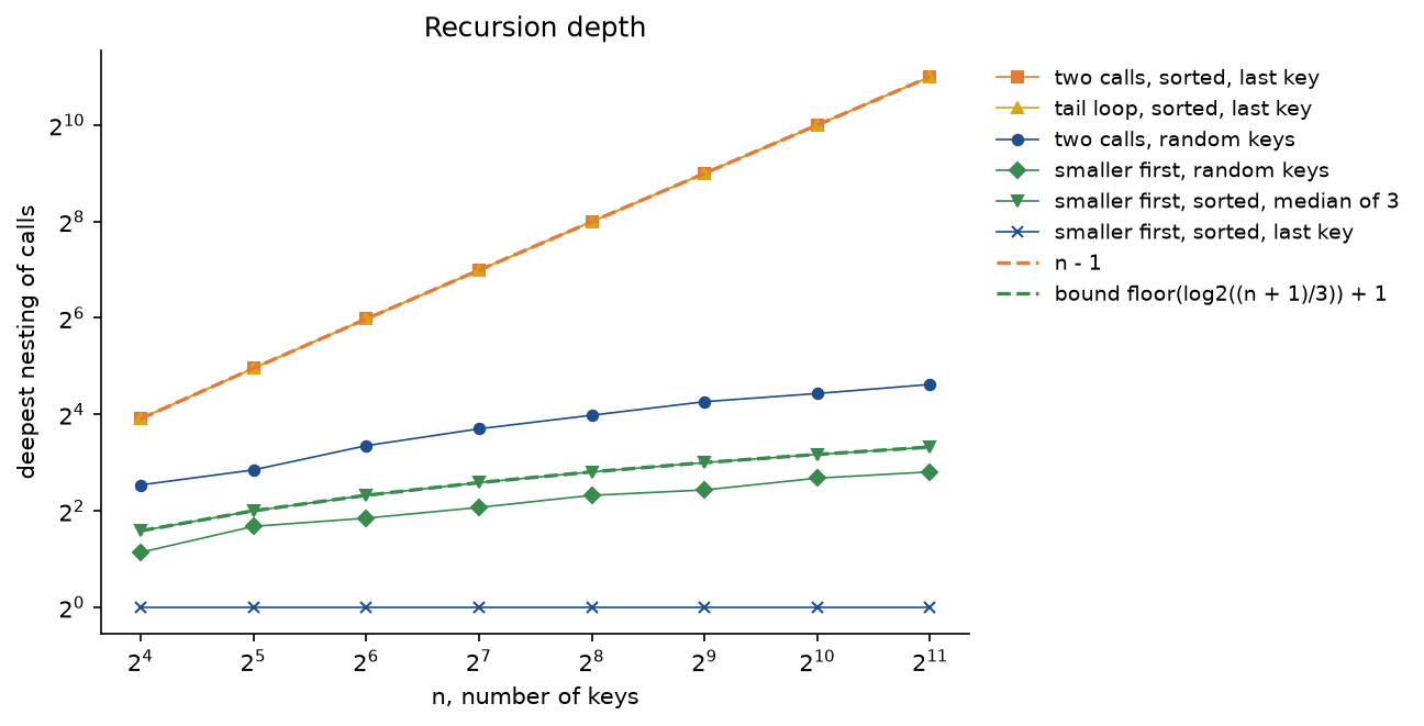
Sorted input with the last key nests 2047 calls deep at n = 2048 with two calls per partition, and exactly as deep with the tail call looped, because the part left to the call is the large one. Recursing on the smaller part brings the same quadratic run down to a single frame, since the smaller part is always empty. The bound of the smaller-first recursion is reached exactly by the median of three on sorted keys, whose splits are perfectly balanced: 10 frames for 2048 keys. On random keys the plain recursion reached 24.6 frames on average and the smaller-first one 7.0.

The cutoff measured¶

The example worst_case_and_depth.py sorts 10000 random keys with the median of three and a cutoff M from 0 to 64:

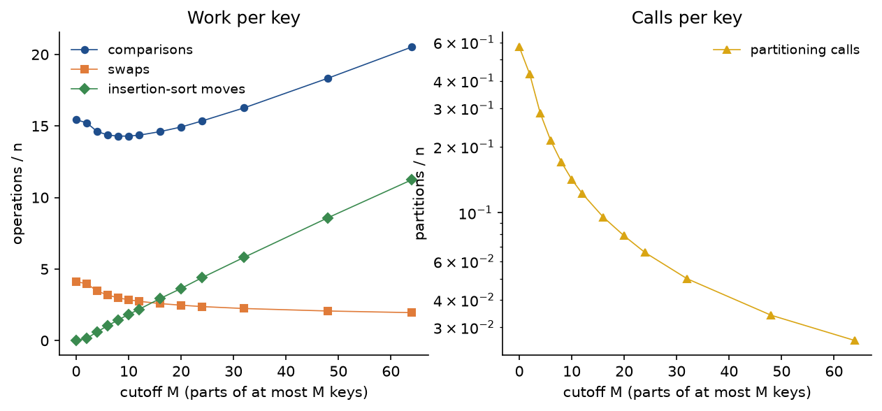
Two panels against the cutoff M from 0 to 64. Left, work per key: comparisons fall from 15.4 at M equal 0 to a minimum of 14.3 near M equal 8 and rise to 20.5 at M equal 64; swaps fall from 4.2 to 2.0; insertion-sort moves rise from 0 to 11.2. Right, partitioning calls per key on a log axis fall from 0.57 at M equal 0 to 0.10 at M equal 16 and 0.026 at M equal 64

Comparisons per key fall from 15.4357 without a cutoff to 14.2876 at M = 8, because the median of three costs three comparisons per partition and tiny partitions are its most expensive use, and rise again beyond about M = 10 as insertion sort's quadratic cost takes over. Partitioning calls drop six-fold by M = 16, from 0.5712 to 0.0955 per key. What the right M is depends on how expensive a call and a move are compared with a comparison, which is a property of the machine, not of the algorithm. In this pure-Python implementation a cutoff of 16 took roughly 0.7 of the time of no cutoff, a rough figure that varies from run to run.

The adversary measured and introsort's guarantee¶

The example builds McIlroy's input against each variant and sorts it with that variant:

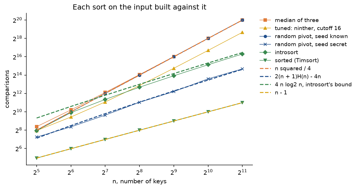
Against the median of three the adversary forced 1053693 comparisons for 2048 keys, 0.2512 n², and replaying the input it built repeated the run exactly. The ninther and a cutoff only lower the constant: 415837. A random pivot with a seed the adversary knew fared no better, 1048783, while the same input sorted with a different seed took 26217, an ordinary random run. Introsort, attacked the same way, took 80803 comparisons, under 4n log2 n = 90112, by switching once to heapsort when its depth limit was exceeded. Timsort is a different story altogether: this adversary is built to catch a pivot, and against a merge sort its answers simply make the input one ascending run, which Timsort finishes in n − 1 comparisons.

Against the lower bound¶

No comparison sort can beat log2 n! comparisons in the worst case, or on average over random inputs, because it must distinguish n! orders:

log2 of n factorial equals n log2 n minus n log2 e plus O of log n, which is about n log2 n minus 1.4427 n

Randomized quicksort's average is within a factor 2 ln 2 = 1.3863 of this bound as n grows, 1.32 at n = 16384, and Python's sorted is within 1.0111 of it on random keys at the same size. Why quicksort is nevertheless often faster in time is a matter of constants other than comparisons: sequential scans, few data moves with Hoare's scheme, no extra memory. The bound itself is derived in The sorting lower bound and linear-time sorts.

Worked example¶

Every step below is printed by examples/worked_example.py and asserted by tests/test_worked_example.py. The keys are the eight integers 46, 86, 20, 93, 23, 37, 63 and 60, whose sorted order is 20, 23, 37, 46, 60, 63, 86, 93.

Lomuto's partition around the last key¶

The pivot is A[7] = 60, i starts at −1 and j walks from 0 to 6:

j = 0: 46 ≤ 60, so i moves to 0 and A[0] is swapped with itself: [46, 86, 20, 93, 23, 37, 63, 60].
j = 1: 86 > 60, nothing moves.
j = 2: 20 ≤ 60, i moves to 1, swap A[1] = 86 and A[2] = 20: [46, 20, 86, 93, 23, 37, 63, 60].
j = 3: 93 > 60, nothing moves.
j = 4: 23 ≤ 60, i moves to 2, swap A[2] = 86 and A[4] = 23: [46, 20, 23, 93, 86, 37, 63, 60].
j = 5: 37 ≤ 60, i moves to 3, swap A[3] = 93 and A[5] = 37: [46, 20, 23, 37, 86, 93, 63, 60].
j = 6: 63 > 60, nothing moves.
Place the pivot: swap A[4] = 86 and A[7] = 60: [46, 20, 23, 37, 60, 93, 63, 86], and return q = 4.

Seven comparisons, one per key other than the pivot, and five swaps, one of them a slot with itself. The pivot 60 is at index 4, its place in the sorted order.

Hoare's partition around the first key¶

The pivot is A[0] = 46, i starts at −1 and j at 8:

Round 1: j moves left past 60 and 63 and stops at A[5] = 37 ≤ 46; i stops at once at A[0] = 46 ≥ 46. Swap them: [37, 86, 20, 93, 23, 46, 63, 60].
Round 2: j stops at A[4] = 23; i stops at A[1] = 86. Swap: [37, 23, 20, 93, 86, 46, 63, 60].
Round 3: j passes 93 and stops at A[2] = 20; i passes 20 and stops at A[3] = 93. Now i = 3 > j = 2: the scans have crossed and the call returns j = 2.

Ten comparisons and two swaps. The parts are A[0..2] = [37, 23, 20] and A[3..7] = [93, 86, 46, 63, 60], every key of the first at most every key of the second, and the pivot 46 sits at index 5 although its sorted place is 3: it will be moved by the recursion on the right part. The placed variant, scanning A[1..7] and swapping the pivot into A[j] at the end, gives [23, 37, 20, 46, 93, 86, 63, 60] with the pivot final at index 3, in 9 comparisons and 3 swaps.

The whole sort¶

Lomuto's quicksort with the last key as pivot, as drawn in the recursion tree above:

Depth 1: partition A[0..7] around 60 as traced, leaving [46, 20, 23, 37] and [93, 63, 86].
Depth 2: partition A[0..3] = [46, 20, 23, 37] around 37: 46 stays, 20 and 23 are swapped forward, and 37 is placed at index 2, giving [20, 23, 37, 46]. Three comparisons and three swaps.
Depth 3: partition A[0..1] = [20, 23] around 23: one comparison and two swaps of a slot with itself.
Depth 2: partition A[5..7] = [93, 63, 86] around 86: 93 stays, 63 is swapped forward and 86 placed at index 6, giving [63, 86, 93]. Two comparisons and two swaps.

The whole sort takes 4 partitions, 13 comparisons and 12 swaps, and the deepest call is at depth 3. Hoare's scheme with the first key as pivot sorts the same keys with 7 partitions, 40 comparisons and only 7 swaps, and nests 5 deep, because after the first round its right part starts with 93, the largest key, and the following pivots are poor.

Three-way partition of keys with repeats¶

The keys 41, 77, 41, 18, 90, 41, 25, 77, 41 are partitioned around the first, 41, with lt = 0, i = 1 and gt = 8:

A[1] = 77 is greater: swap it with A[8] = 41 and move gt to 7: [41, 41, 41, 18, 90, 41, 25, 77, 77]. Two comparisons.
A[1] = 41 is equal: i moves to 2. Two comparisons.
A[2] = 41 is equal: i moves to 3. Two comparisons.
A[3] = 18 is less: swap it with A[0] and move lt and i: [18, 41, 41, 41, 90, 41, 25, 77, 77]. One comparison.
A[4] = 90 is greater: swap with A[7] = 77, gt moves to 6: [18, 41, 41, 41, 77, 41, 25, 90, 77]. Two comparisons.
A[4] = 77 is greater: swap with A[6] = 25, gt moves to 5: [18, 41, 41, 41, 25, 41, 77, 90, 77]. Two comparisons.
A[4] = 25 is less: swap with A[1], lt moves to 2 and i to 5: [18, 25, 41, 41, 41, 41, 77, 90, 77]. One comparison.
A[5] = 41 is equal: i moves to 6, past gt = 5, and the pass ends. Two comparisons.

Fourteen comparisons and five swaps. The result has lt = 2 and gt = 5: A[0..1] = [18, 25] is less than 41, A[2..5] holds all four 41s, finished, and A[6..8] = [77, 90, 77] is greater. Only the two outer parts are sorted further.

Pivot rules on sorted keys¶

The sorted keys 12, 24, 35, 47, 58, 69, 71 with Lomuto's partition:

With the last key as pivot every partition leaves the left part one key shorter and the right part empty: splits 6/0, 5/0, 4/0, 3/0, 2/0 and 1/0, 21 = 7 · 6/2 comparisons, and calls nested 6 deep.
With the median of three, the samples 12, 47 and 71 are already in order, so the three ordering steps exchange nothing, 47 is the pivot and is swapped into the last slot: [12, 24, 35, 71, 58, 69, 47]. The partition splits 3/3, and the two parts split 1/1 each: 19 comparisons, 9 of them spent on samples, and calls nested only 2 deep.

At seven keys the median of three barely pays for its samples; at 2048 keys the same two rules differ by a factor of 97 in comparisons, as the cost section measured.

Instability¶

The records 7a, 3a, 7b, 5a, 3b, 5b compared by number only come out of Lomuto's quicksort as 3a, 3b, 5a, 5b, 7b, 7a. The first partition, around 5b, swaps 7a with 3a, then 7a with 5a, which carries 7a past 7b, then 7b with 3b, and finally 7a with the pivot, which leaves 7a at the end, behind 7b. Sorting the pairs (number, input position) instead gives 3a, 3b, 5a, 5b, 7a, 7b, the stable order that sorted returns.

The code¶

The package quicksort is plain Python, one idea per module. Importing it needs only the standard library; Matplotlib is imported by plotting.py alone.

counting.py holds OperationCounter, with the fields comparisons, swaps, moves, partitions and fallbacks, which every sort accepts as an optional counter; DepthGauge, the high-water mark of the recursion; and CountedKey, a wrapper that counts the less-than tests library code makes.
primitives.py holds less and swap, the counted comparison and the counted, traced exchange that everything else is written with.
trace.py holds the Step record (action, positions, keys, array snapshot, range, scan indices, outcome), record, describe and format_trace, which turns steps into the lines printed above.
lomuto.py, hoare.py and three_way.py hold the partitions: lomuto_partition, hoare_partition, hoare_placed_partition and three_way_partition.
pivots.py holds the pivot rules, with median_of_three, order_three, ninther, choose_pivot and place_pivot.
engine.py holds the four schemes behind one interface, partition_step, and quicksort, the configurable sort on an explicit stack with its three ways of organising the recursion; recursive.py holds the same sort written as real recursion, quicksort_recursive and quicksort_smaller_first.
insertion.py and heapsort.py hold the two helpers on subarrays, and introsort.py holds introsort with its depth_limit.
adversary.py holds McIlroy's Adversary, the Probe stand-ins and killer_input.
analysis.py holds every closed form and recurrence of the cost section; variants.py names the configurations that the examples and the project compare.
invariants.py holds partition_violation, is_partitioned, check_partition, the sorted checks and the loop invariants of the three schemes, which the tests check after every step of traced runs.
workloads.py holds the worked example's keys and seeded inputs: permutations, keys with repeats, sorted, reversed, organ pipe, nearly sorted, few distinct values and adversarial ones.
frames.py turns traces into the states of a partition and the tree of calls of a sort; drawing.py draws the states as rows of cells pinned at computed positions, layout.py places the tree of calls with a tidy tree layout, and tree_drawing.py draws it.
comparisons.py puts Python's sorted next to the package; pitfalls.py holds deliberately broken versions for the pitfalls below; plotting.py draws every plot in the handbook's colours.

Counting and tracing never change what the code does; a test sorts the same keys with and without them. The examples run in seconds each from the repository root:

examples/worked_example.py prints every step of the worked example and writes the four generated diagram sources.
examples/expected_comparisons.py checks the pair probabilities, the swap and partition counts, the expected comparisons and their spread.
examples/worst_case_and_depth.py measures the worst case and its remedies, the recursion depth and the insertion-sort cutoff.
examples/equal_keys_and_adversary.py measures equal keys and three-way partitioning, McIlroy's adversary and introsort.
examples/common_mistakes.py runs every broken version from pitfalls.py next to the correct code.
examples/compare_with_sorted.py checks every variant against sorted and counts both on six kinds of input.
examples/practice.py prints fresh exercises with their solutions; --seed gives a new set.

python searching-and-sorting/quicksort/examples/worked_example.py
python searching-and-sorting/quicksort/examples/expected_comparisons.py
python searching-and-sorting/quicksort/examples/worst_case_and_depth.py
python searching-and-sorting/quicksort/examples/equal_keys_and_adversary.py
python searching-and-sorting/quicksort/examples/common_mistakes.py
python searching-and-sorting/quicksort/examples/compare_with_sorted.py
python searching-and-sorting/quicksort/examples/practice.py --seed 7

The sample project, project/sort_bench.py with its helpers project/bench_inputs.py and project/bench_runner.py, is a test bench for sorting routines. It runs the eight variants of variants.py and Python's sorted over inputs modelled on data programs really sort: shuffled identifiers, an append-only log already in time order, the same log newest first, response status codes with eight values of very unequal frequency, a temperature curve that rises and falls (an organ pipe), events listed in arrival order although stamped when they were sent (nearly sorted, with local disorder), and McIlroy's adversary built against each sort in turn. It reports comparisons and swaps per n log2 n and the deepest nesting of calls, lists the runs that went quadratic and saves two figures. The default run sorts 2000 keys with three seeds per random input and takes about 10 seconds; --size, --seeds, --variants and --inputs change the setup and --figures writes the PNGs elsewhere.

python searching-and-sorting/quicksort/project/sort_bench.py
python searching-and-sorting/quicksort/project/sort_bench.py --size 4000 --variants "median of three,introsort,sorted"

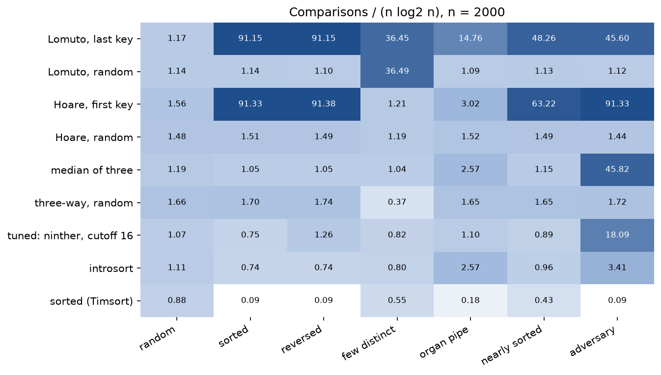
Every dark cell is a quadratic run, and the grid says which defence covers which input. A random pivot fixes ordered inputs and the adversary but not repeated keys, where Lomuto's scheme fails whatever the pivot: 36.5 n log2 n on status codes. Hoare's stopping scans fix repeated keys; three-way partitioning turns them into an advantage, 0.37 n log2 n. The median of three fixes ordered inputs but falls to its adversary, 45.8 n log2 n, and so does the tuned quicksort with a ninther, at 18.1. Only introsort has no dark cell, its worst being 3.4 n log2 n against its own adversary. Timsort, the reference, is in a class of its own on ordered and nearly ordered inputs, finding the runs that quicksort ignores.

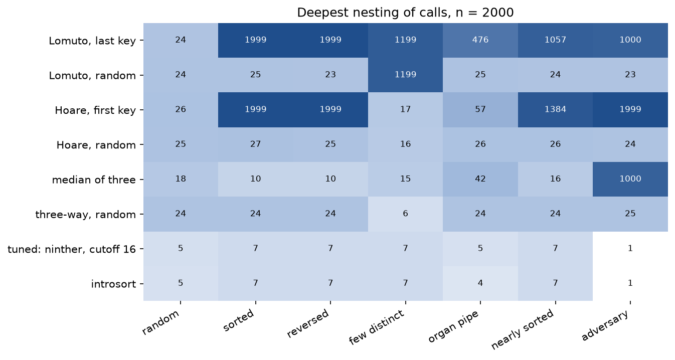
The depth grid mirrors the comparison grid for the plain recursions: a quadratic run is also a deep one, 1999 frames for 2000 sorted keys, far beyond Python's limit and deep enough to overflow a thread's stack in C. The two variants that recurse on the smaller part never nest more than 7 calls deep, on every input including the quadratic adversary run of the tuned quicksort.

The notebook quicksort.ipynb follows this page: both partitions traced, the recursion tree, pivot rules on sorted keys, the randomized analysis checked by counting, equal keys, the stack depth, the adversary and a short run of the bench. The tests in tests check the worked example value by value, the loop invariants after every step of traced partitions, every scheme, rule, recursion order and cutoff against sorted on random inputs with repeats, the formulas against exact recurrences and measured means, the adversary's replay, and the broken versions, and run in a few seconds:

python -m pytest searching-and-sorting/quicksort

All data are synthetic, generated from seeds by workloads.py and project/bench_inputs.py, so nothing is downloaded and no licence is involved.

In practice¶

Python's sorted¶

Python's sorted and list.sort do not use quicksort at all. They use Timsort, a stable merge sort that finds the ascending and descending runs already present in the data and merges them, with the merge order chosen by the Powersort rule since Python 3.11. Every variant in the package agrees with it on numbers, strings and tuples, and comparisons can be counted on both sides by wrapping each key, which is how sorted_counted works:

from quicksort import BY_NAME, OperationCounter, random_permutation, sorted_counted

keys = random_permutation(4096, seed=3)
result, timsort = sorted_counted(keys)
counter = OperationCounter()
ours = BY_NAME["introsort"].sort(list(keys), counter)
assert ours == result
print(timsort / len(keys), counter.comparisons / len(keys))

On 4096 random keys sorted made 10.70 comparisons per key, the median of three 13.97 and introsort 13.17. On sorted and reversed keys sorted made exactly one comparison per key, finding a single run, while introsort made 9.06 and the median of three 12.50; on nearly sorted keys sorted made 1.96. Only with few distinct values did a quicksort win: three-way partitioning made 5.24 comparisons per key against 6.72. In wall-clock time sorted, written in C, was roughly 25 to 35 times faster than the package's introsort in this pure-Python implementation, the ratio varying from run to run, a gap that says nothing about the algorithms and everything about the languages.

Stability and keys¶

sorted is stable, so sorting records by one field keeps the order of an earlier sort by another, and a key function costs one call per item, not per comparison. A quicksort can be made stable only by making keys unique, sorting (key, position) pairs as stable_quicksort does, at the cost of an extra comparison on ties and the memory for the pairs.

Elsewhere¶

Quicksort survives in the unstable sorts of systems languages, always engineered along the lines of this page:

C++'s std::sort is introsort in the major standard libraries: a median-of-three quicksort with a depth limit of about 2 log2 n, a heapsort fallback and an insertion-sort pass for small parts; std::stable_sort is a merge sort.
Go's sort package has used pdqsort, pattern-defeating quicksort, since Go 1.19, and slices.Sort uses it too: introsort plus detection of already sorted parts and of many equal keys, switching to a partition that puts equal keys aside, and shuffling a few keys when splits stay bad.
Rust's sort_unstable used pdqsort and was replaced by ipnsort in Rust 1.81, again a quicksort hybrid; its stable sort is driftsort, a merge sort.
Java's Arrays.sort on primitive arrays has used Yaroslavskiy's dual-pivot quicksort since Java 7, which partitions into three parts around two pivots; on objects, where stability is required, it uses Timsort.
NumPy's np.sort with its default kind, named quicksort, is an introsort, and its stable kind is a radix sort or Timsort depending on the type.

The common thread is that nobody ships the textbook version. The pivot comes from a median of several samples or a ninther, ties are handled by stopping scans or three-way partitions, small parts go to insertion sort, the smaller part is sorted first, and a depth limit or a randomized fallback removes the quadratic case. Modern implementations also avoid unpredictable branches in the partition loop, because on current processors a mispredicted comparison costs more than the comparison itself.

When to use which:

Use sorted or list.sort in Python, always: stable, adaptive to runs, and implemented in C.
Use introsort, or your standard library's unstable sort, when you need an in-place sort without extra memory and do not need stability.
Use three-way partitioning when keys repeat heavily, and a radix sort when keys are small integers or fixed-length strings.
Use merge sort when stability or a guaranteed O(n log n) with sequential access matters, for example on linked lists or external data.
Use quickselect, the partition with one recursive call, when you need the k-th smallest key rather than a sorted array; it is the subject of Selection and order statistics.
Never sort untrusted input with a deterministic quicksort that has no depth limit.

Pitfalls¶

Mixing the return conventions of Lomuto and Hoare. Lomuto returns the pivot's final index q, so the recursion is on [lo, q − 1] and [q + 1, hi]; Hoare's original returns a boundary j, so it is on [lo, j] and [j + 1, hi]. Recursing on [lo, j − 1] and [j + 1, hi] after Hoare's scheme leaves A[j] unsorted: the keys 42, 55, 98, 93, 77, 13, 69 come out as 13, 42, 69, 77, 93, 55, 98. Recursing on [lo, q] and [q + 1, hi] after Lomuto's scheme never ends when the pivot is the largest key. examples/common_mistakes.py runs this and every following mistake.
Taking Hoare's pivot from the last slot. With the pivot in A[hi] and that key the largest, the scans return j = hi, the right part is empty and the left part is the whole range again: the sort never finishes. Move the chosen pivot to A[lo] first.
Starting Lomuto's index at lo. The small region is empty at the start, so i must be lo − 1. Starting at lo leaves A[lo] unexamined on the small side, and a large key there stays in front.
Choosing a pivot but not moving it into the slot the scheme reads. Partitioning around the median's value while A[hi] stays in place makes the final swap put the wrong key between the regions.
Advancing i in three-way partitioning after a swap with gt. The key that arrives from gt has not been examined; skipping it leaves a 77 among the 41s in the worked example.
Scanning past keys equal to the pivot. Scans that skip equal keys sort correctly but split n equal keys n − 1 against 0: 523776 comparisons for 1024 equal keys, against 9218 when the scans stop on them.
Finding the median of three without ordering the samples. Swapping the median into place and leaving the other two samples where they were made reversed input quadratic with the placed Hoare partition: 134394 comparisons for 1024 reversed keys, against 10761 when the samples are put in order first.
Trusting the plain recursion with sorted input. On 3000 sorted keys with the last key as pivot it raises RecursionError in Python. Looping on the tail call alone does not help, the recursion would still nest 2999 deep; recurse on the smaller part and the depth is 1.
Using a random pivot with a seed others know. McIlroy's adversary built against seed 42 forced 262466 comparisons on 1024 keys; the same keys took 11906 with another seed. Seed from the system, or use introsort.
Expecting stability. Equal keys can change order: 7a, 3a, 7b, 5a, 3b, 5b becomes 3a, 3b, 5a, 5b, 7b, 7a. Sort (key, position) pairs or use a stable sort.
Using Lomuto's scheme on data with many repeats, whatever the pivot rule: status codes with eight values made 36.5 n log2 n comparisons in the bench, against 1.2 for Hoare's scheme.
Measuring with correlated randomness. Drawing the input and the pivots from generators with the same seed made the smallest and largest of 10 keys meet in 29 percent of the runs instead of 20. Use separate seeds, or keep the input fixed and vary only the pivots.
Tracing by hand: when tracing Hoare's scheme, write down where each scan stops before swapping, and remember that both stop on keys equal to the pivot; when tracing Lomuto's, remember the swaps of a slot with itself, which are counted, and that the pivot is placed at i + 1, not at i.