B-trees and B+ trees

A balanced binary search tree finds a key among a million in about twenty steps, and in memory that is fast enough. On a disk or an SSD, where every step reads a page of several kilobytes and a read costs as much as many thousands of comparisons, twenty reads per lookup is far too many. B-trees fix this by making every node as wide as a page: a node holds hundreds of keys in order and has hundreds of children, so a million keys fit in a tree of height 2 and a billion in a tree of height 3 or 4. This page builds multiway search trees and B-trees from scratch, states the node size rules in both common conventions, inserts keys bottom-up and top-down and deletes them with borrowing and merging, traced key by key, then turns the B-tree into the B+ tree that databases use, with all records in linked leaves and cheap range scans. It counts every page read and write with a simulated pager to show why a fan-out in the hundreds wins, bulk loads trees from sorted input, checks every invariant after long random operation sequences, and compares the code with sortedcontainers, whose SortedList is close to a B+ tree of sorted lists, and with the B-trees inside SQLite. Afterwards you will be able to trace any insertion or deletion by hand at any order, convert between the two conventions without slips, predict the height and the page reads of a tree, and choose between a B-tree, a B+ tree, a sorted container and a log-structured design for a real workload. It builds on Binary search trees, and the balanced binary trees it is measured against are AVL trees and Red-black trees.

The structures need only the standard library; to run the plots and the notebook install the base group, and the structures group for the comparison with sortedcontainers. SQLite comes with Python.

Intuition

Picture a large library that keeps its catalogue cards in a basement store. Fetching a drawer from the store takes a minute; reading the cards in a drawer you already hold takes a second. A binary catalogue, in which every drawer holds a single card that says "smaller titles to the left, larger to the right", would need twenty trips to the basement to find one title among a million. A sensible librarian does the opposite: each drawer holds several hundred cards in order, each card says where the drawer for the titles between it and the next card is, and the top drawer always stays on the desk. Two or three trips find any title, and each drawer is read from front to back while you hold it, which costs almost nothing.

That catalogue is a B-tree. It keeps the comparisons of a binary search, about log2 n of them, but packs them into a few wide nodes so that the expensive operation, fetching a node, happens only a few times. It stays balanced by a simple rule: every drawer except the top one stays at least half full, and all the bottom drawers sit at the same depth. When a drawer overflows it splits in two and passes one card up; when it runs too empty it borrows a card from a neighbour or merges with it.

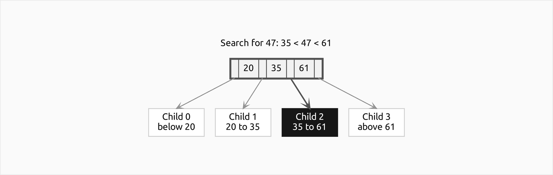
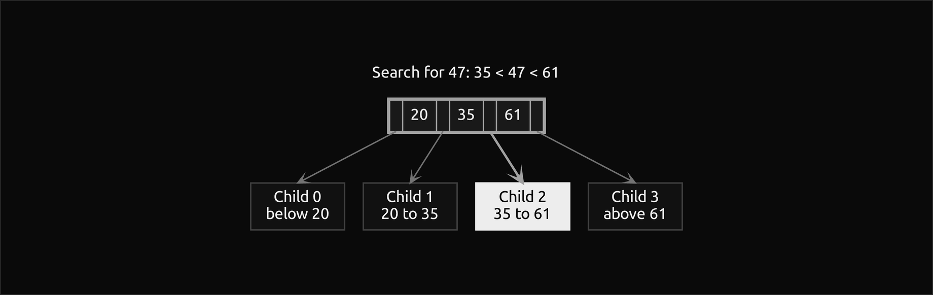
A node with three keys has four children, one for each gap between and around its keys. A search compares the key it is looking for with the keys of the node, finds the gap it falls into and follows that one pointer, drawn thicker here, into the filled child.

How it works

Height, order and minimum degree

Height counts the edges on the longest path from the root down to a leaf, as everywhere in this handbook: a tree whose root is a leaf has height 0 and the empty tree has height -1. A lookup reads one node per level, so it reads height + 1 nodes.

Two conventions name the size of B-tree nodes, and mixing them up is the most common error with B-trees. Knuth's order m is the largest number of children a node may have, so a node holds at most m − 1 keys. The minimum degree t, used by Cormen, Leiserson, Rivest and Stein, is the smallest number of children a node other than the root must have. They describe the same trees whenever m is even: a B-tree of minimum degree t is exactly a B-tree of order m = 2t.

In the minimum-degree convention the same limits read:

The rest of this page always speaks of the order m and gives t in brackets where it exists. Order 3 allows 1 or 2 keys per node (2-3 trees), order 4 allows 1 to 3 keys (minimum degree 2, the 2-3-4 trees behind red-black trees), order 5 allows 2 to 4 keys and order 6 allows 2 to 5 keys (minimum degree 3). The odd orders have no minimum degree at all. The package keeps the rule in one place, the Order object, which answers max_keys, min_keys, max_children, min_children and minimum_degree, and Order.from_minimum_degree(t) converts the other convention. The minimum is "half full, rounded up" for the children: ⌈m/2⌉ children and ⌈m/2⌉ − 1 keys. Reading "half" as m/2 keys is wrong for every even order; for order 4 it demands 2 keys where 1 is legal.

Multiway search trees

A multiway search tree of order m generalises a binary search tree. Every node holds up to m − 1 keys in increasing order and has one child slot for every gap between and around them, and every key in a child lies strictly between the two keys that frame its slot:

Search starts at the root, finds the slot of the key by comparing it with the node's keys, and either stops when it meets the key or follows the slot; an empty slot ends an unsuccessful search. Nothing more is promised, and that is the problem. The simple insertion rule, put the key into the node where the search ends if it has room, otherwise hang a new node in the empty slot, never splits anything, so keys that arrive in sorted order build a chain:

The plain multiway tree on the left has height 4 for nine keys and would have height n / 2 for n keys, as bad as a linked list. The B-tree on the right holds the same keys at height 2 because of the two rules that follow.

The B-tree

A B-tree of order m is a multiway search tree with two more invariants:

• Every node other than the root holds between ⌈m/2⌉ − 1 and m − 1 keys; the root holds at least 1 key unless the tree is empty. An internal node with k keys has exactly k + 1 children.
• All leaves are at the same depth.

The second rule makes the tree perfectly balanced in height, and the first makes it bushy, so the height is logarithmic with base about m/2. A tree of height h holds the most keys when every node is full, and the fewest when the root holds one key and every other node is at its minimum of d − 1 keys, with d = ⌈m/2⌉:

The fewest keys come from the sparsest tree:

Both bounds count edges. Taken together, the height of every B-tree of n keys is Θ(log n / log m):

check_btree tests both invariants together with the search order, walking the tree with an explicit stack and carrying the range of keys each node may hold; it raises with a sentence that names the first node that breaks a rule. Passing another order to it checks a drawn tree against a label: a tree that has a node with three keys cannot be a B-tree of order 3, whatever its caption says.

Search

Search is the multiway search above: in each node, a binary search over the keys finds the key or the child whose range contains it, and a leaf ends an unsuccessful search. It visits height + 1 nodes at most, each one a page read on a cold cache. The binary search inside a node costs about log2 m comparisons, so the whole lookup costs about (h + 1) log2 m ≈ log2 n comparisons, no fewer than a balanced binary tree makes. A B-tree does not save comparisons; it saves page reads.

Insertion, bottom-up

A new key always goes into a leaf: search for it, and put it into the leaf where the search ends, in order. That keeps every leaf at the same depth. If the leaf now holds m keys, one too many, it splits: the middle key moves up into the parent, the keys before it stay in the left half and the keys after it go to a new right sibling. The parent gains one key and one child, and if it overflows in turn it splits the same way. A split of the root makes a new root holding the single key that moved up, and that is the only way a B-tree grows taller, so all leaves stay level.

The two halves are always legal, because an overfull node of m keys splits into a left half of ⌈(m − 1)/2⌉ keys, the key that moves up and a right half of ⌊(m − 1)/2⌋ keys, and the smaller half still meets the minimum:

For an odd order the overfull node holds an odd number of keys and its middle is unique. For an even order the overfull node holds m keys, an even number, and there are two middle keys; either one leaves both halves legal, and the choice is a convention that changes the tree. This page moves the upper middle key up, the key at index m // 2, which leaves the extra key in the left half; BTree(order, median="lower") takes the key before it instead. When you trace an insertion by hand, decide the convention first and keep it.

The highlighted nodes, drawn with a thick outline and shaded cells, received the key that moved up, and the filled key is the one just inserted; in the frame before 66 they are the full leaf and the full root that the insertion is about to split. The last frame is the cascade: the new key overflows its leaf, the key that moves up overflows the parent, and the tree grows a level.

Insertion, top-down in one pass

Bottom-up insertion walks down to a leaf and then possibly all the way back up. The single-pass variant avoids the return trip by splitting early: on the way down, before stepping into a child that is full, split that child, and split the root first if it is full. The parent always has room for the key that moves up, because the parent was itself split if it was full, so no split ever propagates. The new key then goes into a leaf that cannot overflow.

This needs an even order. A full node of order 2t holds 2t − 1 keys, an odd number, and splits around its exact middle into two halves of t − 1 keys, the minimum:

For an odd order a full node holds m − 1 keys, an even number, and splitting it before it overflows leaves one half below the minimum:

That is why the single-pass method belongs to the minimum-degree convention, and why insert_top_down refuses an odd order. Top-down insertion pays for its single pass with splits that bottom-up insertion would not have made: it splits every full node it passes, even when the leaf below has room.

The same fourteen keys, the same order, a different tree: top-down insertion splits each full node as it passes it, so its splits happen one insertion earlier than the overflows that bottom-up insertion waits for, and they pick different middle keys.

Deletion

Deletion must keep both invariants too, and it works on leaves just like insertion:

• A key in an internal node is first replaced by its in-order predecessor, the largest key of the child just before it, which always sits in a leaf; the predecessor is removed from that leaf instead. The in-order successor, the smallest key of the child just after it, works equally well. No key of the tree lies between the deleted key and either replacement, so the search order survives, but the two choices give different trees, both valid. This page uses the predecessor; delete(key, replacement="successor") uses the other.
• If the leaf still holds at least ⌈m/2⌉ − 1 keys, nothing else happens.
• Otherwise the node is underfull, and it borrows: if a sibling next to it holds more than the minimum, the separator between them in the parent comes down into the underfull node and the sibling's nearest key goes up to replace it, with the sibling's nearest child moving across too when the nodes are internal. This rotation through the parent keeps the order, because the separator lies between the two siblings' keys.
• If neither sibling can spare a key, the node merges with a sibling and the separator between them into one node. The parent loses a key and a child and may become underfull itself, so the repair moves up.
• When the root loses its last key, its only child becomes the root and the tree gets one level shorter, the only way a B-tree shrinks.

A merge never overfills a node: the underfull node holds d − 2 keys, the sibling that could not spare one holds d − 1, and with the separator that makes 2d − 2 ≤ m − 1:

The order of the attempts is a convention as well: this package tries to borrow from the left sibling, then from the right one, and merges with the left sibling when there is one. A sibling is only read, and charged a page read, when the code asks it.

The highlighted node is where each deletion ended: the leaf that lost 26, and the leaf that gave up 48 to replace 55, which still holds the minimum of one key. The next four deletions each leave a node underfull and need a repair:

The highlighted node is the one each repair ended in: the parent whose separator changed after a borrow, the merged leaf after a merge, and the new root after the cascade. The last deletion shows the whole cascade: the leaf merges with its sibling, which empties the parent, which merges with its own sibling and takes the root's only key, and the empty root disappears.

B+ trees

A B-tree stores records in every node, so an internal node spends most of its page on values that a search only passes through. A B+ tree separates the two jobs:

• Every record, key and value, lives in a leaf, and the leaves are linked left to right into a sorted list.
• Internal nodes hold only separator keys and child pointers. Child j holds the keys from separator j up to but not including separator j + 1, so a key equal to a separator belongs to the right.
• A leaf has its own capacity L, usually different from the internal order m, because a page holds fewer records than separators. A leaf other than the root holds between ⌈L/2⌉ and L records.

Insertion goes to a leaf as before. A full leaf splits into two leaves of about equal size, the new leaf is linked in after the old one, and the first key of the right leaf is copied up as the new separator: the record stays in the leaf, because records live only there. An overfull internal node splits exactly like a B-tree node, and its middle key moves up and leaves the node. Copy up for leaves, move up for internal nodes: copying at an internal split would leave a node with as many keys as children, and moving at a leaf split would lose the record.

Every lookup ends in a leaf, even when the key equals a separator on the way down, so a point lookup in a B+ tree is never shorter than in a B-tree of the same height; the gain lies elsewhere. A range query from low to high descends once to the leaf that can hold low and then follows the leaf links, reading each further leaf once and never going back up the tree, and it stops at the first key above high.

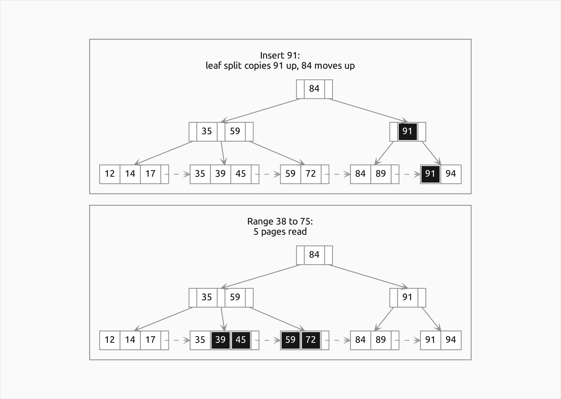
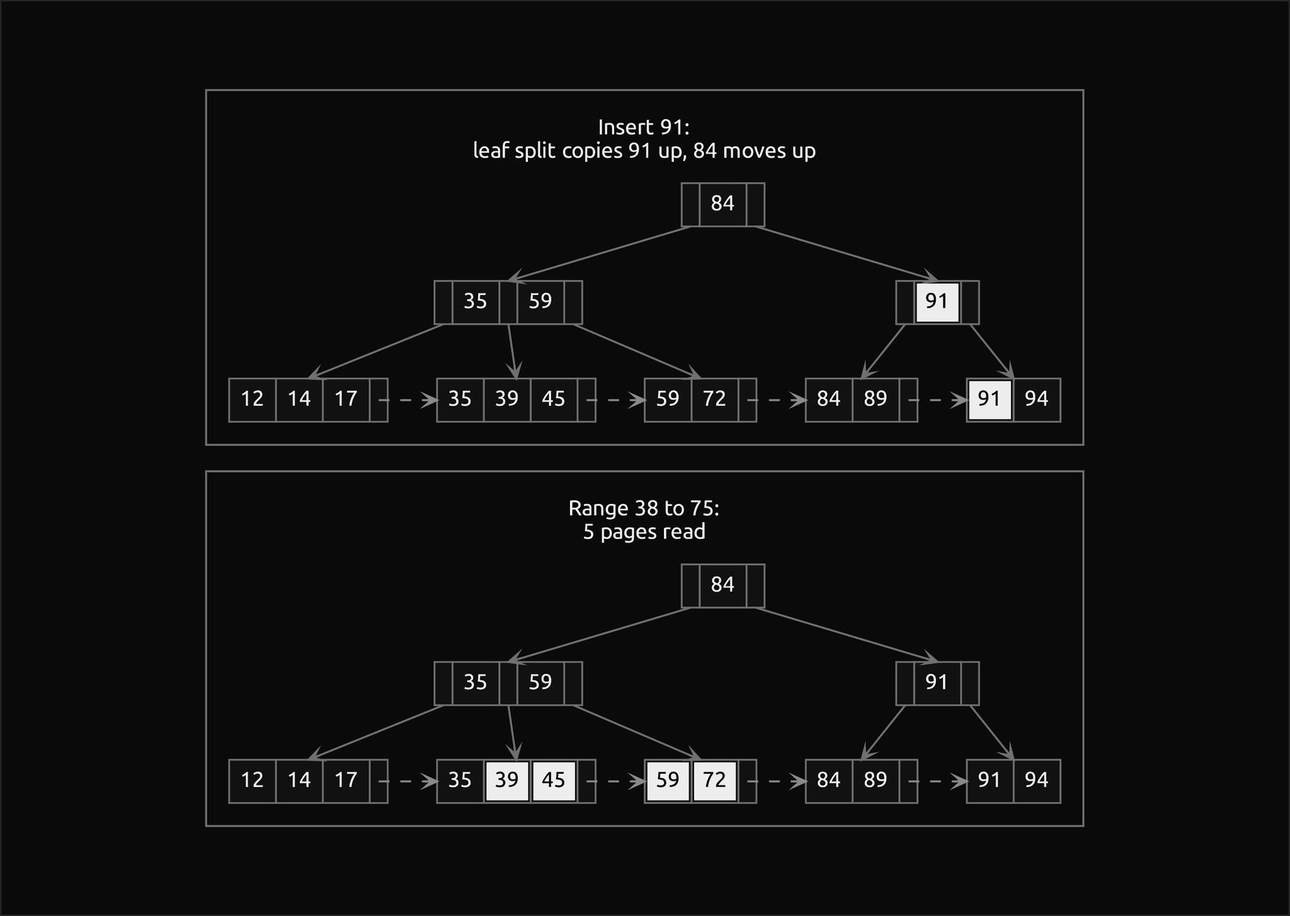
The dashed arrows are the leaf links. The range scan reads the root, the internal node [35, 59] and three leaves, five pages in all: it walks from the leaf [35, 39, 45] to [59, 72] and stops in [84, 89] at the first key above 75.

Deletion removes the record from its leaf. A leaf below its minimum borrows one record from a sibling that can spare one, and the separator between them becomes the first key of the right-hand leaf of the pair; otherwise the two leaves merge, the chain skips the leaf that disappears, and the separator leaves the parent. Internal nodes are repaired as in a B-tree. A separator may outlive its record: after a deletion it may name a key that is no longer in any leaf, and that is fine, because it still bounds the keys on both sides correctly. Only a lookup that stops at the separator, instead of going down to the leaf, gets it wrong.

In the last frame the root holds 84 although the record 84 was deleted: a stale separator, still correct as a bound.

Bulk loading

Building a tree from n sorted records by n insertions splits nodes over and over and writes most pages many times. Bulk loading builds the tree from the bottom up instead, the way an index is built over a sorted file. For a B+ tree, cut the records into runs of about f·L records, where f is the fill factor, make each run a leaf and link the leaves; then group the leaves into internal nodes of about f·m children, with the smallest key of every child but the first as separators, and group those nodes again until one node, the root, remains. For a B-tree the leaves hold runs of keys with one key held back between neighbouring leaves; the held-back keys become the key sequence of the next level up. In both cases partition cuts each level into groups as even as possible, and uses fewer, larger groups when even groups would fall below the minimum.

Every page is written exactly once, no node is searched or split, and every node is as full as asked. A fill of 1 makes the shortest possible tree for read-only data; a fill below 1 leaves room in every leaf for later insertions, which otherwise would split almost every leaf of a full tree.

The disk model

Every node is one page, and the package counts what a database would pay for it through a Pager. A tree tells the pager when it visits a node and when it changes one. A visit to a page in the pager's least-recently-used cache is a hit and costs nothing; any other visit is a page read and brings the page into the cache. With cache_pages=0 every visit is a read, which is the cost of an isolated lookup. Writes are charged per operation: each changed page, including a new one, is written once when the operation ends, as a database that makes every change durable at once would. Counting never changes a result, and every number in the next section is a count of these page reads and writes, so it is the same on every machine.

Cost

Every operation

For a B-tree of order m holding n keys, with height h = Θ(log n / log m):

• Search: at most h + 1 page reads and about log2 n comparisons, worst case.
• Insertion, bottom-up: h + 1 page reads on the way down and 1 + 2s page writes for an insertion that makes s splits, because each split writes the new right node and the parent. A single insertion can split once per level, Θ(h) in the worst case, but splits are rare on average, as below.
• Deletion: h + 1 page reads to find the key and its replacement, plus up to two sibling reads per level that needs repair, and a small number of writes per repaired level; Θ(h) in the worst case.
• Range query of k keys: about h + 1 + k / ℓ page reads, with ℓ the mean number of records per leaf, for a B+ tree or a B-tree read with a cursor that keeps its path.
• Bulk loading n sorted records: one write per page, about n / L page writes in all, and no reads.

All of these are worst-case bounds of order h; nothing is amortized except the remark that splits are rare. Because h is so small, three or four for any data set that fits on one machine, the difference between best and worst case lies almost entirely in which pages the cache already holds.

Height

The bounds of the previous section hold for every insertion order. The example disk_costs.py inserts random permutations of 16 to 16384 keys into B-trees of order 3, 8 and 64 and records the height:

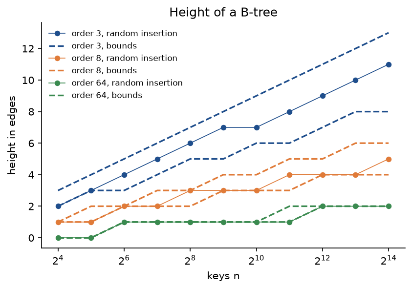
The measured heights stay inside the bounds, and closer to the lower one, because random insertion leaves nodes about two thirds full rather than at the minimum. Order 64 holds 16384 keys at height 2, three levels; a 2-3 tree needs 11 edges.

Page reads and the order

Page size decides the order. A node of order m holds m − 1 keys of k bytes and m pointers of p bytes plus a header of H bytes, and must fit in a page of P bytes:

With 4096-byte pages and 8-byte keys a node has order 255, and the height bounds give height 2 for a million keys and 3 to 4 for a billion, so 3 and 4 or 5 page reads, against 20 and 30 for a perfectly balanced binary tree with one node per page. The ratio between the two is the base of the logarithm:

A binary tree laid out perfectly balanced reads one page per level, about this many on average:

The example measures both, with a cold cache (cache_pages=0) and with a warm least-recently-used cache:

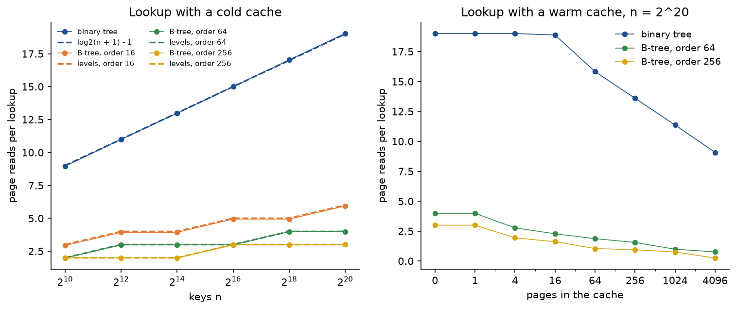
At n = 2^20 a cold lookup reads 19.0370 pages in the binary tree, against 5.9365, 3.9870 and 2.9985 for orders 16, 64 and 256, each just below its number of levels because the few keys stored in internal nodes are found before the leaves. The right panel shows the second advantage of wide nodes: their top levels are tiny. The two upper levels of the order-256 tree are a handful of pages, so a 64-page cache brings a lookup down to 1.0433 reads, essentially the leaf alone, while 4096 cached pages still leave the binary tree at 9.0812 reads, because only the top twelve of its twenty levels fit in the cache. The comparisons do not improve: at n = 2^16 a lookup makes 18.4870 comparisons in the order-256 tree and 18.8530 at order 64, against 22.9990 in the binary tree, which tests twice per level; all are close to log2 n = 16 plus one equality test per level.

Records stored in the nodes cost fan-out. With 100-byte records in 4096-byte pages a B-tree node has order 38, while a B+ tree keeps order 255 for its internal nodes and puts 40 records in each leaf. For 262144 records the B-tree is 3 edges high and a cold lookup reads 4.0000 pages; the B+ tree is 2 high, uses 6581 pages against 7087 and reads 3.0000. For a billion records the bounds give heights 5 to 6 for the B-tree against 4 for the B+ tree.

Splits, writes and fill

Every split creates one node, so a tree of N nodes has had fewer than N splits, and the minimum fill bounds N:

So a split happens at most once every d − 1 insertions, amortized, even though one unlucky insertion can split every level. Random insertion does better than this worst case: the nodes settle at about ln 2 of their capacity on average, a classical result for random insertion, so the tree has about n / ((m − 1) ln 2) nodes:

The example insertion_costs.py measures both for 16384 random keys and orders 4 to 256, and the fill against n:

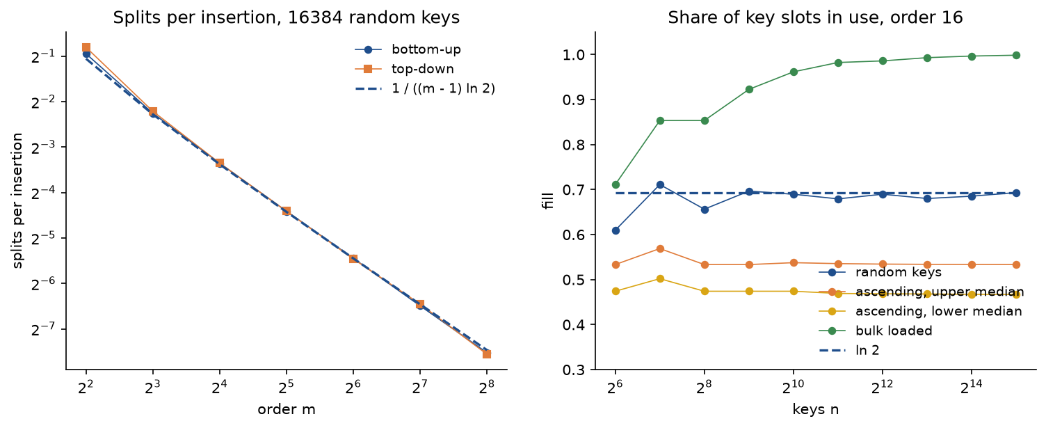
Bottom-up insertion split 0.0977 times per insertion at order 16 against the predicted 0.0962, and 0.0054 times at order 256 against 0.0057; at order 4 the prediction, which assumes wide nodes, is less accurate, 0.5187 against 0.4809. Pages written per insertion follow from 1 + 2s: 2.0375 at order 4, 1.1954 at order 16 and 1.0109 at order 256, so with real page sizes almost every insertion writes exactly its leaf. The fill at n = 32768 and order 16 was 0.6933 for random keys, next to ln 2 = 0.6931. Ascending keys are worse: every split leaves a left half that never receives another key, so the nodes end about half full, 0.5333 with the upper median and 0.4670 with the lower one, and bulk loading fills them, 0.9984. Top-down insertion pays for its early splits on small orders: for 4096 random keys at order 4 it made 2320 splits against 2157 and built a tree of height 8 against 7; from order 16 on the two are indistinguishable.

Range scans

A range of k keys costs one descent and then about one leaf per ℓ records:

The example scans_and_bulk_loading.py inserts 65536 random keys into a B+ tree and a B-tree of order 64 and answers ranges of 1 to 4096 keys with an empty cache:

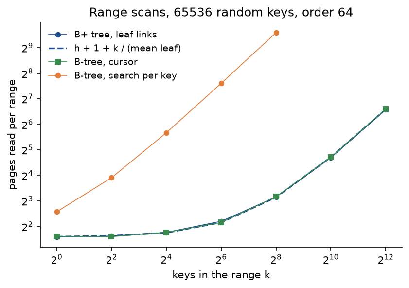
The B+ tree read 3.00 pages for one key, 8.90 for 256 and 95.28 for 4096, close to the prediction with 44.0726 records per leaf. The B-tree read through a cursor that keeps its path on a stack costs the same, 8.95 and 96.92 pages: in page reads alone the leaf links buy nothing that a careful cursor cannot do. What they buy is simplicity and locality: the cursor of a B+ tree is a single leaf pointer instead of a stack of h nodes, a scan never revisits the upper levels or holds them, and the records it returns are packed in leaves with no separators between them. What neither structure can afford is answering a range one key at a time with a fresh search for each successor: 771 page reads for 256 keys.

Bulk loading

Bulk loading writes each page once, about n / L leaf pages plus a geometric series for the levels above:

The example measures it against insertion for leaf capacities from 4 to 128 records:

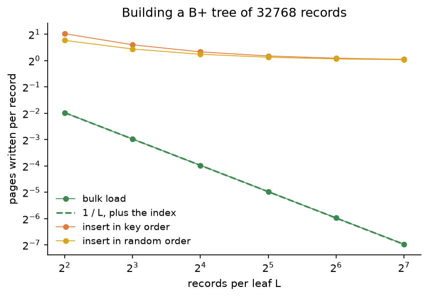
For 32768 records and leaves of 128 records, bulk loading wrote 0.0080 pages per record against 1.0320 for inserting the records in key order and 1.0235 in random order, about 130 times fewer, and filled every leaf, where insertion in key order left the leaves half full (0.5010) and random insertion 0.6772 full.

Worked example

Every step below is printed by examples/worked_example.py and asserted by tests/test_worked_example.py. The B-tree has order 4, which is minimum degree t = 2: every node other than the root holds 1 to 3 keys and has 2 to 4 children. The keys are inserted in the order 26, 42, 70, 55, 76, 56, 78, 43, 24, 86, 58, 48, 15 and 66. A split of an overfull node of four keys moves its upper middle key, the third, up.

Inserting bottom-up, key by key

• 26, 42 and 70 go into the root, which is a leaf: [26, 42, 70]. Each insertion reads and writes one page.
• 55: the leaf becomes [26, 42, 55, 70], four keys, one too many. It splits: 55 moves up into a new root [55], leaving the leaves [26, 42] and [70]. The tree grows from height 0 to height 1. One page read, three pages written (the old leaf, the new leaf and the new root).
• 76 goes to the right leaf, [70, 76]; 56 too, [56, 70, 76].
• 78: the right leaf becomes [56, 70, 76, 78] and splits; 76 moves up, the root becomes [55, 76] over [26, 42], [56, 70] and [78].
• 43 joins the left leaf, [26, 42, 43].
• 24: the left leaf becomes [24, 26, 42, 43] and splits; 42 moves up, the root becomes [42, 55, 76] over [24, 26], [43], [56, 70] and [78].
• 86, 58, 48 and 15 each fit into their leaves: [78, 86], [56, 58, 70], [43, 48] and [15, 24, 26]. The root and the leaf [56, 58, 70] are now full.
• 66 belongs between 58 and 70: the leaf becomes [56, 58, 66, 70] and splits, and 66 itself moves up. The root becomes [42, 55, 66, 76], four keys, and splits too: 66 moves up again, into a new root [66], over [42, 55] and [76]. Two page reads, five pages written.

The final tree has height 2: the root [66], the internal nodes [42, 55] and [76], and the leaves [15, 24, 26], [43, 48], [56, 58], [70] and [78, 86]. The fourteen insertions made 5 splits, 24 page reads and 24 page writes. With the lower middle key moving up instead, the same keys give a tree of height 1, the root [42, 56, 76] over the leaves [15, 24, 26], [43, 48, 55], [58, 66, 70] and [78, 86]; both trees are valid, which is why a trace must state its convention.

Inserting top-down

The single-pass method inserts the same keys into the tree of minimum degree 2 and splits every full node it passes:

• 26, 42 and 70 fill the root leaf, [26, 42, 70].
• 55: the root is full, so it splits before the descent: 42 moves up into a new root [42], over [26] and [70]. Then 55 goes into [55, 70]. Two page reads, three writes.
• 76 joins [55, 70, 76], which is now full but stays whole until an insertion passes through it.
• 56: the descent meets the full leaf [55, 70, 76] and splits it first: 70 moves up, the root becomes [42, 70] over [26], [55] and [76], and 56 goes into [55, 56].
• 78, 43, 24 and 86 fit: [76, 78], [43, 55, 56], [24, 26] and [76, 78, 86].
• 58: the full leaf [43, 55, 56] splits on the way down, 55 moves up, the root becomes [42, 55, 70], and 58 goes into [56, 58].
• 48: the root [42, 55, 70] is full and splits first, so 55 moves up into a new root [55] over [42] and [70]; 48 then goes into [43, 48]. Three page reads, four writes.
• 15 and 66 fit: [15, 24, 26] and [56, 58, 66].

The result, [55] over [42] and [70] over the leaves [15, 24, 26], [43, 48], [56, 58, 66] and [76, 78, 86], has height 2 like the bottom-up tree but different nodes, after 4 splits instead of 5. No split ever travelled back up: each happened before the descent continued.

Searching

Search for 58 in the bottom-up tree: in the root [66], 58 < 66, so take the first child; in [42, 55], 58 > 55, so take the third child; the leaf [56, 58] holds 58. Search for 50 follows [66], then [42, 55], where 42 < 50 < 55 selects the middle child, and ends in the leaf [43, 48] without finding it. Each search reads 3 pages and makes 6 comparisons: a binary search over each node and one equality test.

Deleting

The six deletions start from the bottom-up tree and use the predecessor, borrow from the left sibling before the right one, and merge only when neither sibling can spare a key:

• Delete 26: the leaf [15, 24, 26] keeps two keys, [15, 24], more than the minimum of 1. Three page reads, one write.
• Delete 55: it sits in the internal node [42, 55]. Its predecessor is the largest key of the child before it, 48 in [43, 48]; 48 replaces 55, giving [42, 48], and the leaf keeps [43]. Three reads, two writes.
• Delete 43: its leaf becomes empty, below the minimum. The left sibling [15, 24] can spare a key, so the separator 42 comes down into the empty leaf, 24 goes up into the parent, which becomes [24, 48], and the siblings are [15] and [42]. Four reads, because the left sibling was read too, and three writes.
• Delete 70: its leaf [70] is the first child of [76], so there is no left sibling; the right sibling [78, 86] can spare a key. The separator 76 comes down, 78 goes up, the parent becomes [78] and the siblings [76] and [86]. Four reads, three writes.
• Delete 15: its leaf empties; it is the first child of [24, 48], and its right sibling [42] holds only the minimum. They merge with the separator 24 into [24, 42], and the parent keeps [48], still legal. Four reads, two writes, one merge.
• Delete 76: its leaf empties, and its right sibling [86] holds only the minimum, so they merge with the separator 78 into [78, 86]. The parent [78] is now empty, below the minimum; its left sibling [48] cannot spare a key either, so they merge with the root's separator 66 into [48, 66]. The root has lost its only key, so its only child [48, 66] becomes the root, and the tree shrinks to height 1 over the leaves [24, 42], [56, 58] and [78, 86]. Five reads, two writes, two merges.

With the successor instead, the deletion of 55 (after 26) takes 56 from the leaf [56, 58], leaves [42, 56] above [43, 48] and [58], and is just as valid.

The B+ tree

The B+ tree has internal order 4 and leaves of at most 3 records, at least 2 below the root. The keys 14, 84, 17, 59, 72, 35, 94, 89, 45, 12, 39 and 91 are inserted, each with a short label as its value:

• 14, 84 and 17 fill the root leaf, [14, 17, 84].
• 59: the leaf becomes [14, 17, 59, 84] and splits into [14, 17] and [59, 84]; 59 is copied up into a new root [59] and stays in its leaf.
• 72 and 35 fit: [59, 72, 84] and [14, 17, 35].
• 94: [59, 72, 84, 94] splits into [59, 72] and [84, 94], and 84 is copied up: the root is [59, 84].
• 89 fits, [84, 89, 94]; 45 overflows [14, 17, 35, 45], which splits into [14, 17] and [35, 45], and 35 is copied up: the root is [35, 59, 84].
• 12 and 39 fit: [12, 14, 17] and [35, 39, 45].
• 91: [84, 89, 91, 94] splits into [84, 89] and [91, 94], and 91 is copied up into the root, which becomes [35, 59, 84, 91] with five children, one too many. The internal node splits around its middle key, and 84 moves up, leaving the node: [35, 59] and [91] under a new root [84]. Two page reads, five writes.

The range scan from 38 to 75 reads the root [84] (38 < 84, first child), the internal node [35, 59] (35 ≤ 38 < 59, second child) and the leaf [35, 39, 45], which yields 39 and 45; it follows the link to [59, 72], which yields 59 and 72, and to [84, 89], where 84 > 75 ends the scan. Five page reads return four records.

The deletions:

• Delete 35: the leaf keeps [39, 45], the minimum. The separator 35 stays in [35, 59] although the record is gone; every key to its right is still at least 35.
• Delete 45: the leaf [39] is below the minimum, and the left leaf [12, 14, 17] can spare a record. 17 moves across, giving [12, 14] and [17, 39], and the separator becomes 17, the new first key of the right leaf: [17, 59].
• Delete 14: the leaf [12] is below the minimum and is the first child; its right sibling [17, 39] holds only the minimum, so the two leaves merge into [12, 17, 39] and the separator 17 leaves the parent, which becomes [59].
• Delete 84: the leaf [89] is below the minimum and merges with [91, 94] into [89, 91, 94], so the separator 91 leaves its parent, which is left with one child, below the minimum of two. Its left sibling [59] has only two children, so the two internal nodes merge with the root's separator 84 into [59, 84], and the empty root disappears. The new root [59, 84] holds 84 as a separator although the record 84 is gone, as a bound for [89, 91, 94].

The code

The package b_trees is plain Python, one idea per module. Importing it needs only the standard library; Matplotlib is imported by plotting.py alone, and sortedcontainers and sqlite3 inside the functions of comparisons.py.

• order.py holds Order, the node size rules with the order m and the minimum degree t, Order.from_minimum_degree and median_index, which picks the key that moves up.
• counting.py holds OperationCounter, with the fields comparisons, page_reads, page_writes, splits, borrows and merges, ensure_counter and CountedKey, which counts the comparisons library code makes.
• pager.py holds Pager, the least-recently-used page cache that charges page reads and writes.
• nodes.py holds the node classes Node, Leaf and Internal, and the counted binary searches inside a node, find_slot and route.
• trace.py holds the Step record, record, describe and format_trace, which print the traces above.
• multiway.py holds MultiwayTree, the unbalanced multiway search tree.
• btree.py holds BTree with search, iteration and the queries; insertion.py holds insert_bottom_up and insert_top_down, and deletion.py the deletion with borrow_from_left, borrow_from_right and merge_children.
• bplus.py holds BPlusTree with lookups and insertion with copy-up and move-up splits; bplus_deletion.py holds its deletion.
• bulk.py holds bulk_load_btree, bulk_load_bplus and partition; scans.py holds the range queries: the B+ tree's scan along its leaves, and the B-tree's with a cursor and with one search per key.
• disk.py holds the page arithmetic fan_out, the height bounds, PagedBinaryTree and mean_page_reads.
• invariants.py holds btree_violation, bplus_violation and multiway_violation with is_ and check_ versions.
• workloads.py holds the worked examples' keys and seeded random inputs and operation sequences.
• layout.py computes a tidy layout of a multiway tree: subtrees side by side as close as their outlines allow, each node over its children with its pointers above them; it also holds path_of, which finds the node that holds a key. cells.py builds the row of key and pointer cells that draws one node. drawing.py pins every node at its position and returns deterministic Graphviz text for one tree, a before and after pair, or rows of frames that fit the width of a card.
• comparisons.py puts sortedcontainers and SQLite next to the package; pitfalls.py holds deliberately broken versions for the pitfalls below; plotting.py draws every figure in the handbook's colours.

Counting and tracing never change what the code does. The heart of bottom-up insertion is a short loop over the recorded path:

while len(node.keys) > tree.order.max_keys:
    middle = median_index(len(node.keys), tree.median)
    promoted, right = split_node(tree, node, middle)
    grew = not path
    if grew:
        parent, index = tree.new_node(children=[node]), 0
        tree.root = parent
    else:
        parent, index = path.pop()
    parent.keys.insert(index, promoted)
    parent.children.insert(index + 1, right)

The examples run in a few seconds each from the repository root:

• examples/worked_example.py prints every step of the worked examples and writes the seven generated diagram sources.
• examples/disk_costs.py turns page sizes into orders and measures heights and page reads per lookup.
• examples/insertion_costs.py measures splits, writes and fill for both insertion methods and both median conventions.
• examples/scans_and_bulk_loading.py measures range scans and bulk loading.
• examples/common_mistakes.py runs every broken version from pitfalls.py next to the correct code.
• examples/compare_with_libraries.py checks the package against sortedcontainers and inspects SQLite's B-trees.
• examples/practice.py prints fresh exercises with their solutions; --seed gives a new set.

python trees/b-trees/examples/worked_example.py
python trees/b-trees/examples/disk_costs.py
python trees/b-trees/examples/insertion_costs.py
python trees/b-trees/examples/scans_and_bulk_loading.py
python trees/b-trees/examples/common_mistakes.py
python trees/b-trees/examples/compare_with_libraries.py
python trees/b-trees/examples/practice.py --seed 7

The sample project, project/kv_store.py with its helpers, is a tiny on-disk key-value store: a B+ tree over fixed-size pages in a real file. codec.py lays out the pages, a leaf with sorted 8-byte keys, value slots of 24 bytes and the number of the next leaf, an internal page with separators and 4-byte page numbers; with 4096-byte pages a leaf holds 127 records and an internal page up to 341 children. pagefile.py reads and writes pages with a small least-recently-used write-back cache, which writes a changed page only when it is evicted or flushed, keeps a free list of released pages, and counts the reads and writes that reach the file. disk_tree.py and disk_delete.py hold the B+ tree algorithms of the package rewritten over page numbers, with bulk loading and a check that walks every page; workload.py holds the measurements. The default run creates the file in a temporary directory, bulk loads 200000 records at fill 0.9 (1764 page writes: 1762 node pages and two writes of the header), reopens the file and reads every record back, runs 30000 mixed operations with a 32-page cache, checking every answer against a dict, reopens and checks again, and measures lookups for cache sizes from 0 to 4096 pages. It takes about ten seconds; --records, --operations, --page-size, --cache-pages, --fill and --seed change the setup and --figures writes the figure elsewhere.

python trees/b-trees/project/kv_store.py
python trees/b-trees/project/kv_store.py --page-size 512 --cache-pages 8

The tree has height 2: 1755 leaves under 6 internal pages and a root, 7052 KiB on disk. In the mixed workload a lookup read 1.0011 pages on average, because the 32-page cache holds every internal page and only the leaf has to come from the file, and a range scan of about a hundred records read 1.8718. Writes go to the file only when the cache evicts a changed page, so they land on whichever operation needs the room: 14800 page writes in all, 0.9926 per insertion, update or deletion. To predict the reads of a lookup for any cache size, suppose the cache always held the top of the tree, whole levels from the root down and then part of the next:

The figure compares this prediction with the measured cache:

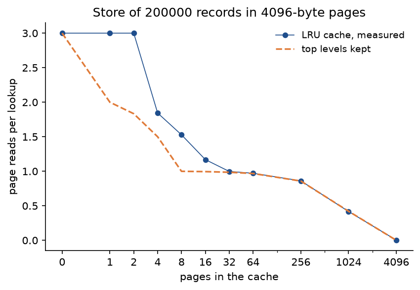
From 32 pages on the least-recently-used cache does as well as the ideal one, 0.9978 against 0.9858 reads at 32 pages and 0.4176 against 0.4205 at 1024. With one or two pages it does nothing at all: every lookup touches three pages in turn, so the root is always the least recently used page when the leaf arrives, and it is evicted just before it is needed again. Real buffer pools pin the root and the upper levels, or use replacement policies that favour frequently used pages, for exactly this reason. The last measurement inserts 10000 new keys into a store of 50000 records: appended after the largest key they cost 0.0162 page writes each, because one cached leaf takes key after key and is written once when it fills; at random places they cost 0.9908, almost a whole page per 32-byte record.

The notebook b_trees.ipynb follows this page: the conventions, the worked examples step by step, the invariants under random operations checked against SortedList, the page reads of binary trees and B-trees plotted, splits and bulk loading, sortedcontainers and SQLite, and a small run of the store. The tests in tests check the worked examples value by value, the invariants after thousands of random operations at several orders with both insertion methods and both conventions, the cost claims on counts, the agreement with sortedcontainers and SQLite, and the project's store, and run in a few seconds:

python -m pytest trees/b-trees

All data are synthetic, generated from seeds by workloads.py and the project, so nothing is downloaded and no licence is involved.

In practice

sortedcontainers

Python's standard library has no sorted map or balanced tree; the usual choice is the sortedcontainers package. Its SortedList keeps the values in a list of sorted Python lists, each between half the load factor and twice the load factor long (1000 by default), and a flat list of the largest value of each sublist above them. That is a B+ tree of height 1 in all but name: the sublists are the leaves, the list of maxima is a single internal level searched with bisect, and a sublist that grows past twice the load splits in half while one that shrinks to half the load merges into its neighbour. Its leaves are lists in memory rather than pages, so splitting is a fast memory copy and the single internal level can grow to tens of thousands of entries without harm. examples/compare_with_libraries.py shows the agreement and the shape:

from sortedcontainers import SortedList

from b_trees import BPlusTree, BTree, random_operations, replay

operations = random_operations(20000, seed=8)
reference = replay(SortedList(), operations)
assert replay(BTree(5), operations) == reference
assert replay(BPlusTree(6), operations) == reference

Every insertion, deletion, membership test and range query of the 20001 operations got the same answer from the three structures. After 100000 random insertions the SortedList held 64 sublists of 1415 to 1708 values, a mean of 1562.5000, and after 100000 ascending ones 99 sublists of 1000 to 2000 values: the same pattern as the B-tree fill above, about 0.7 for random keys and about half for ascending ones. Counted through wrapped keys, 20000 random insertions cost 266490 comparisons in SortedList and 312002 in BTree(64), 13.3245 and 15.6001 per insertion, both close to log2 20000 = 14.2877. In wall-clock time the pure-Python B-tree takes about 6 times as long as SortedList, and SortedList about 8 times as long as a dict, which has no order at all. When to use which:

• Use dict or set when order does not matter, and hash tables in general.
• Use sortedcontainers.SortedList, SortedDict or SortedSet for an ordered collection in memory: range queries with irange, rank queries, both ends.
• Use bisect on a plain list when the data are mostly read and rarely changed.
• Use a B+ tree when the data live on disk, which in Python means a database such as SQLite rather than your own code.
• Use the package's classes to learn and to experiment: they show every split and count every page.

SQLite and other databases

SQLite stores every table and every index of a database file as a B-tree of pages, 4096 bytes by default. Tables with an integer row id are B+ trees, with all row data in the leaves and only row ids in the interior pages; indexes are B-trees whose interior pages hold full keys. The dbstat table shows their shape, and sqlite_index_shape reads it for an index on integer keys inserted in random order. For 100000 rows the index has height 2: a root with 2 children, 2 interior pages with 153.5 children each and 307 leaves of 324.7 keys on average. For 400000 rows it still has height 2, with 211.8 children per interior page (at most 258) and 1271 leaves of 313.7 keys. That is the page arithmetic of this page with real cells: an integer key with its row id takes about a dozen bytes, so a page holds a few hundred of them, and a lookup reads three pages for any table that fits on a laptop. EXPLAIN QUERY PLAN reports SEARCH records USING INDEX records_by_key (key=?) for one key and SEARCH records USING COVERING INDEX records_by_key (key>? AND key<?) for a range, which descends once and then reads the index in key order without touching the table.

PostgreSQL's default index is a B+ tree with linked leaves (a variant by Lehman and Yao that allows concurrent readers and writers), with 8 KB pages, and its index builds sort the data and bulk load it with leaves 90 percent full by default, to leave room for later insertions. MySQL's InnoDB stores each table as a B+ tree on its primary key, with 16 KB pages, so the records are the leaves of the primary index. File systems such as XFS, Btrfs and NTFS keep directories and the maps of file extents in B-trees or B+ trees. Production B-trees also special-case appending: when a row is appended at the end of a table, SQLite starts a new page holding just that row instead of splitting the full page in half, so that ascending keys, the most common insertion order of all, fill pages almost completely instead of half.

Log-structured merge trees

A B-tree updates data in place: every insertion at a random place reads a leaf and writes the whole page back, which in the project cost 0.9908 page writes of 4096 bytes for a 32-byte record, a write amplification of over a hundred, and every write lands at a random position on the device. Log-structured merge trees, introduced by O'Neil and colleagues and used by LevelDB, RocksDB, Cassandra and HBase, make writes sequential instead. New records go into a sorted structure in memory, the memtable, and an append-only log for durability. When the memtable fills, it is written out in one sequential pass as an immutable sorted run, often called an SSTable. Runs accumulate in levels of growing size, and a background compaction merges the runs of a level into the next, exactly the k-way merge of merge sort, dropping overwritten and deleted records on the way; a deletion is just a new record, a tombstone, that hides the older versions.

The price is paid by reads. A lookup must check the memtable and then possibly one run per level, newest first, so each run carries a small index and a Bloom filter that rules out most runs without reading them, and a range scan must merge the streams of all runs. Each record is also rewritten once per level it passes through during compaction, but in long sequential writes. The trade-off is roughly this: B+ trees give the cheapest and most predictable reads and short range scans, and suit read-heavy work and transactions; LSM trees accept slower reads and background work in exchange for much higher write throughput, and suit write-heavy streams such as logs, time series and event stores. Several databases offer both, and RocksDB serves as a storage engine underneath systems that started with B-trees.

Pitfalls

• Mixing the two conventions. "A B-tree of degree 3" means order 3, at most 2 keys per node, in one book, and minimum degree 3, order 6 and at most 5 keys, in another. Convert once, m = 2t, and say which one you use; odd orders exist only in the order convention. examples/common_mistakes.py prints both readings, and runs this and every following mistake.
• Trusting a label. A tree drawn under the caption "order 3" with a node of three keys is not a B-tree of order 3, whatever the caption says; it is a valid tree of order 4. Check the largest and smallest node against the order before tracing. btree_violation(tree, 3) names the node.
• Reading "half full" as m/2 keys. The minimum is ⌈m/2⌉ − 1 keys, ⌈m/2⌉ children. With m // 2 keys as the minimum at order 4, deleting 67 from the tree [67, 75] over [33, 34], [69, 70], [81, 85] triggers a needless merge into [33, 34, 69, 70], four keys in a node that can hold three.
• Splitting on the wrong key. The key that moves up is the middle of the overfull node, including the new key; for even counts pick the upper or the lower middle and keep it. Splitting the node before adding the key, or taking the middle of the old keys, gives a different tree.
• Splitting proactively on an odd order. The single-pass method leaves a node of 1 key in an order-5 tree, below the minimum of 2: inserting 90, 88, 33, 22, 67, 48 and 28 top-down leaves the leaf [90] alone. Use bottom-up insertion for odd orders.
• Forgetting that a split propagates. When the parent was full, it overflows too and splits; when the root splits, a new root appears and the height grows by one. A trace that stops after the leaf split is wrong whenever the parent was full.
• Borrowing from a sibling at its minimum. Borrowing is only allowed from a sibling with keys to spare; otherwise the underflow moves to the sibling, as deleting 98 from the order-4 tree [78, 91] over [15, 21, 60], [86], [98] shows. Merge instead.
• Borrowing past the parent. A key from the sibling never moves straight across: the separator comes down and the sibling's key goes up. Moving 24 straight from [15, 24] into the empty leaf under the separator 42 leaves 24 in the subtree of keys above 42.
• Deleting an internal key like a leaf key. Removing 55 from [42, 55] leaves a node with one key and three children. Replace it by its predecessor or successor from a leaf first; both are correct and give different trees, so a trace must say which.
• Forgetting to shrink the root. When a merge takes the root's last key, the root's only child becomes the root; a root with no keys is not a valid B-tree.
• Copying up at an internal split of a B+ tree, or moving up at a leaf split. Separators are copied up from leaves, because the record must stay in a leaf, and moved up from internal nodes, because an internal node with k keys must have k + 1 children: copying 84 up from [35, 59, 84, 91] leaves the right half with two keys and two children, and moving 91 up from [84, 89, 91, 94] loses the record 91.
• Stopping a B+ tree lookup at a separator. Separators are copies that can outlive their records; after deleting 35 from the worked B+ tree, a lookup that stops at the separator 35 reports a deleted key. Always go down to the leaf.
• Expecting B+ trees to make lookups shorter or scans read fewer pages than a careful B-tree cursor. A point lookup in a B+ tree always reaches a leaf, and a B-tree cursor that keeps its path reads about as many pages for a range. The gains are a higher fan-out when records are large, a trivial cursor and records packed in leaves.
• Answering a range with one search per key. Each successor search descends from the root again: 771 page reads for 256 keys against 8.95 with a cursor or the leaf links.
• Building a multiway tree without balancing. Ascending keys turn it into a chain of height about n / (m − 1): 18 ascending keys give a multiway tree of order 3 height 8 against height 3 for the B-tree.
• Bulk loading unsorted input, or inserting sorted input one key at a time. Bulk loading needs strictly increasing keys and raises otherwise; inserting sorted keys one by one works but leaves nodes half full and, with leaves of 128 records, writes about 130 times as many pages.
• Expecting a unique answer. The median convention, the choice of predecessor or successor and the order of borrowing attempts all change the tree, and every combination is valid. Test the invariants and the contents, not one particular shape.

Further reading

• R. Bayer and E. McCreight, "Organization and maintenance of large ordered indexes", Acta Informatica 1(3), 173-189, 1972. The B-tree.
• D. Comer, "The ubiquitous B-tree", ACM Computing Surveys 11(2), 121-137, 1979. B-trees, B+ trees and their variants in one survey.
• D. E. Knuth, The Art of Computer Programming, volume 3, Sorting and Searching, second edition, section 6.2.4, Addison-Wesley, 1998. Multiway trees and B-trees with the order convention.
• T. H. Cormen, C. E. Leiserson, R. L. Rivest and C. Stein, Introduction to Algorithms, fourth edition, chapter 18, MIT Press, 2022. B-trees with the minimum degree convention and single-pass insertion and deletion.
• A. C.-C. Yao, "On random 2-3 trees", Acta Informatica 9(2), 159-170, 1978. The analysis behind the ln 2 fill of random insertion.
• P. L. Lehman and S. B. Yao, "Efficient locking for concurrent operations on B-trees", ACM Transactions on Database Systems 6(4), 650-670, 1981.
• G. Graefe, "Modern B-tree techniques", Foundations and Trends in Databases 3(4), 203-402, 2011. Bulk loading, fill factors, buffer pools and much more.
• P. O'Neil, E. Cheng, D. Gawlick and E. O'Neil, "The log-structured merge-tree (LSM-tree)", Acta Informatica 33(4), 351-385, 1996.
• A. Petrov, Database Internals, O'Reilly, 2019. B-tree and LSM storage engines side by side.
• The SQLite documentation of the database file format and of the dbstat virtual table.
• The sortedcontainers documentation, in particular its notes on the implementation and on performance at scale.