Merge sort

Merge sort rests on one cheap operation: two lists that are each sorted can be combined into one sorted list by looking only at their two front items, again and again, so the combined list costs one comparison per item at most. Split the input in half, sort each half the same way, merge the halves, and n items are sorted with about n log2 n comparisons in every case, stably, with every item read in sequence. That combination of a guaranteed bound, stability and sequential access is why merge sort sits inside Python's sorted, Java's object sort and every database that sorts more data than fits in memory. This page derives the merge with explicit run ends and its loop invariant, does the sentinel version correctly, builds the top-down and bottom-up sorts, counts their comparisons exactly in the best and worst case, removes the extra copy with alternating buffers, counts inversions on the way, merges the runs already present in the input as Timsort does, sorts a linked list in O(1) extra space, merges k runs with a heap and sorts a file larger than memory. Afterwards you will be able to trace any merge sort by hand split by split and comparison by comparison, predict its exact comparison count, and choose between sorted, heapq.merge and an external sort for a real task. It builds on Elementary sorts and the recurrences of Recurrences, and uses the heap of Heaps and priority queues.

The sorts need only the standard library and the heap package of the heaps topic, which installs with the repository; to run the plots and the notebook install the base group, and add the graphs group for the check against SciPy's Kendall tau.

Intuition

Two people have each sorted half of a pile of returned library books by call number, and the books must go back on one shelf in order. Nobody needs to sort anything again. Look at the first book of each pile, shelve the one with the smaller number, and look again: the next book to shelve is always one of the two now on top. One look per book, never a step back, and when one pile is empty the rest of the other goes on the shelf as it is. That is a merge.

Sorting is then a matter of making sorted piles to merge. A pile of one book is sorted. Two piles of one merge into a sorted pile of two, two of those into a pile of four, and so on: about log2 n rounds of merging, each of which handles every book once. The work barely depends on how the books were arranged: the splitting ignores their order, and every merge passes every book along exactly once.

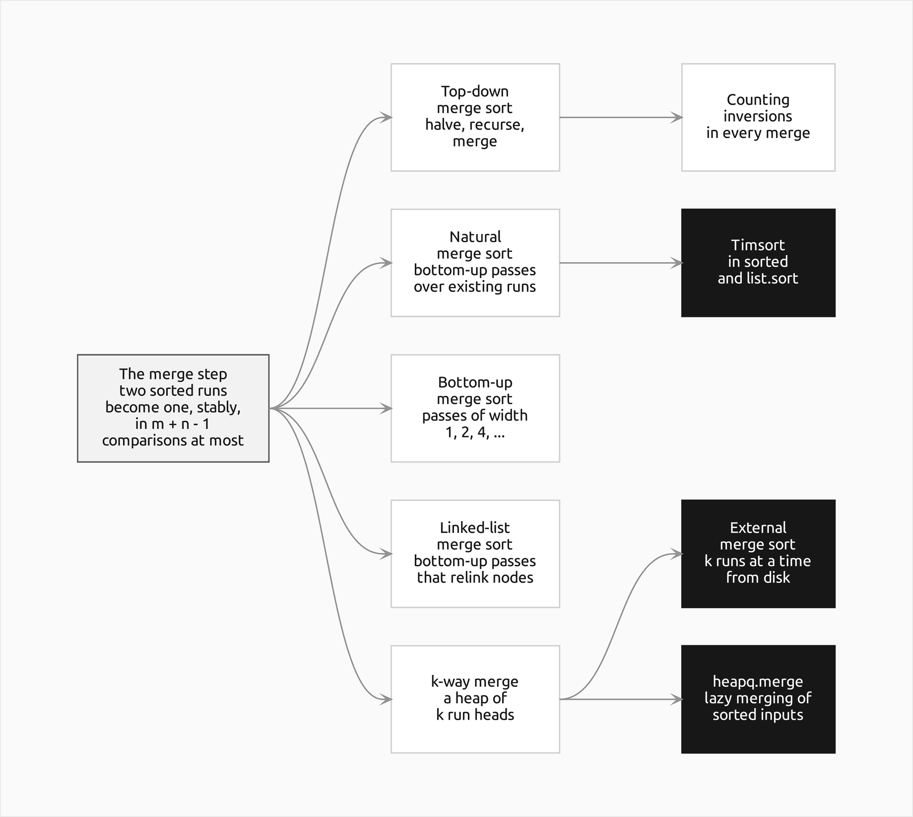
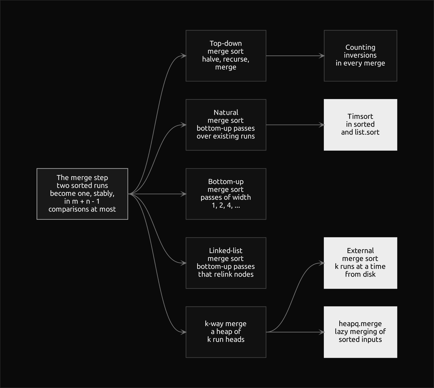
The diagram is a map of this page. Everything grows from the outlined merge step: the two classic sorts, the natural sort that starts from runs already in the data, the linked-list version, and the k-way merge. The filled boxes are the forms you meet in production, Timsort, external sorting and heapq.merge, all of them built on the same merge.

How it works

The merge step

A run is a stretch of items in sorted order. The merge takes two runs that sit side by side in an array, A[lo:mid] and A[mid:hi] in Python's half-open slice notation, and writes their items in sorted order into A[lo:hi] of another array. Keeping the ends half-open is what makes the arithmetic clean: the left run has mid − lo items, the right run hi − mid, and an empty run is simply mid = lo or hi = mid.

The merge keeps three positions: i, the head of the left run, j, the head of the right run, and k, the next slot of the output. While both runs still have items, it compares the two heads, copies the smaller one to slot k and advances that run's head and k. When one run is used up, the rest of the other is copied over without any comparison. The two loop tests, i < mid and j < hi, are the explicit run ends: they are what stops the merge from ever reading past a run.

while i < mid and j < hi:
    counter.comparisons += 1
    took_right = source[j] < source[i]
    if took_right:
        target[k] = source[j]
        j += 1
    else:
        target[k] = source[i]
        i += 1
    k += 1

The merge is correct because of a loop invariant. Writing L for the left run with m items, R for the right run with n items and C for the output:

Initially k = 0 and the statement says nothing. If it holds before an iteration, the smaller of the two heads is no larger than any item still waiting, because each run is sorted, so its head is its smallest remaining item. Placing it keeps C sorted, and it remains no larger than the two heads that follow. When one run is empty, every item of the other is at least the last item placed, and the run is sorted, so copying it across finishes a sorted output. Each iteration places one item, so the loop ends after at most m + n − 1 comparisons. It may end much sooner:

The lower end is reached when every comparison takes an item of the shorter run until that run is used up, for example when every item of the left run is smaller than every item of the right run: merging [1, 2, 3] with [4, 5, 6, 7] takes 3 comparisons. The upper end is reached when the two runs run out together, so that the last two items come from different runs: [1, 3, 5, 7] with [2, 4, 6] takes 6.

The comparison is written source[j] < source[i]: the right item goes first only when it is strictly smaller. On a tie the left item goes first. Since the left run holds items that came earlier in the input, items with equal keys leave the merge in the order they arrived, and merge sort is stable. A stable sort is what lets you sort by one key and then by another and keep the first order among ties, and it is the reason library sorts of objects are merge sorts. Testing source[i] <= source[j] instead is the same rule; reversing it, by taking the right item on ties, still sorts but is no longer stable.

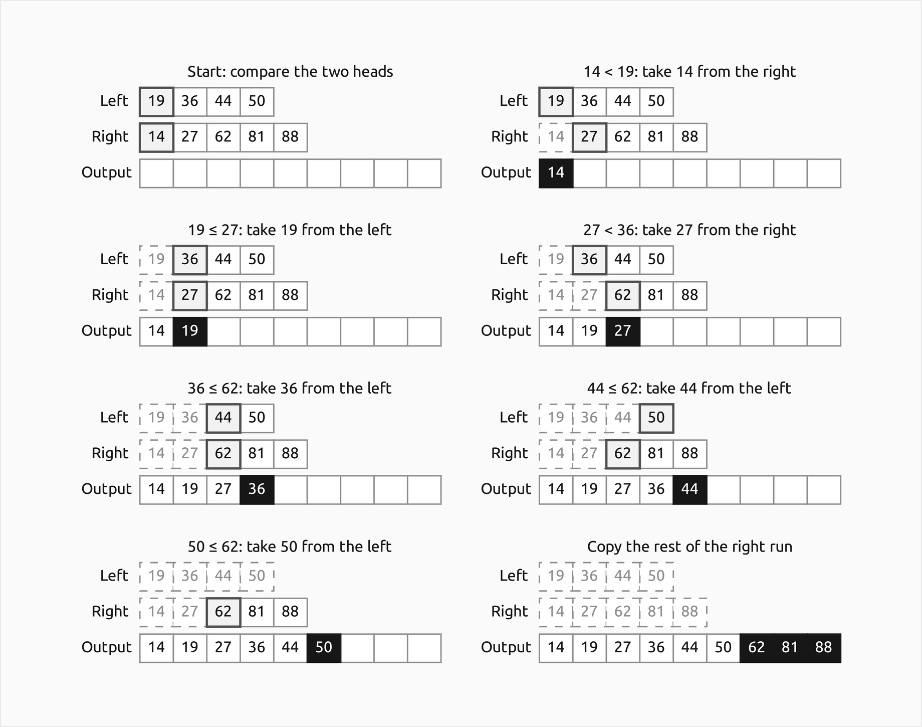
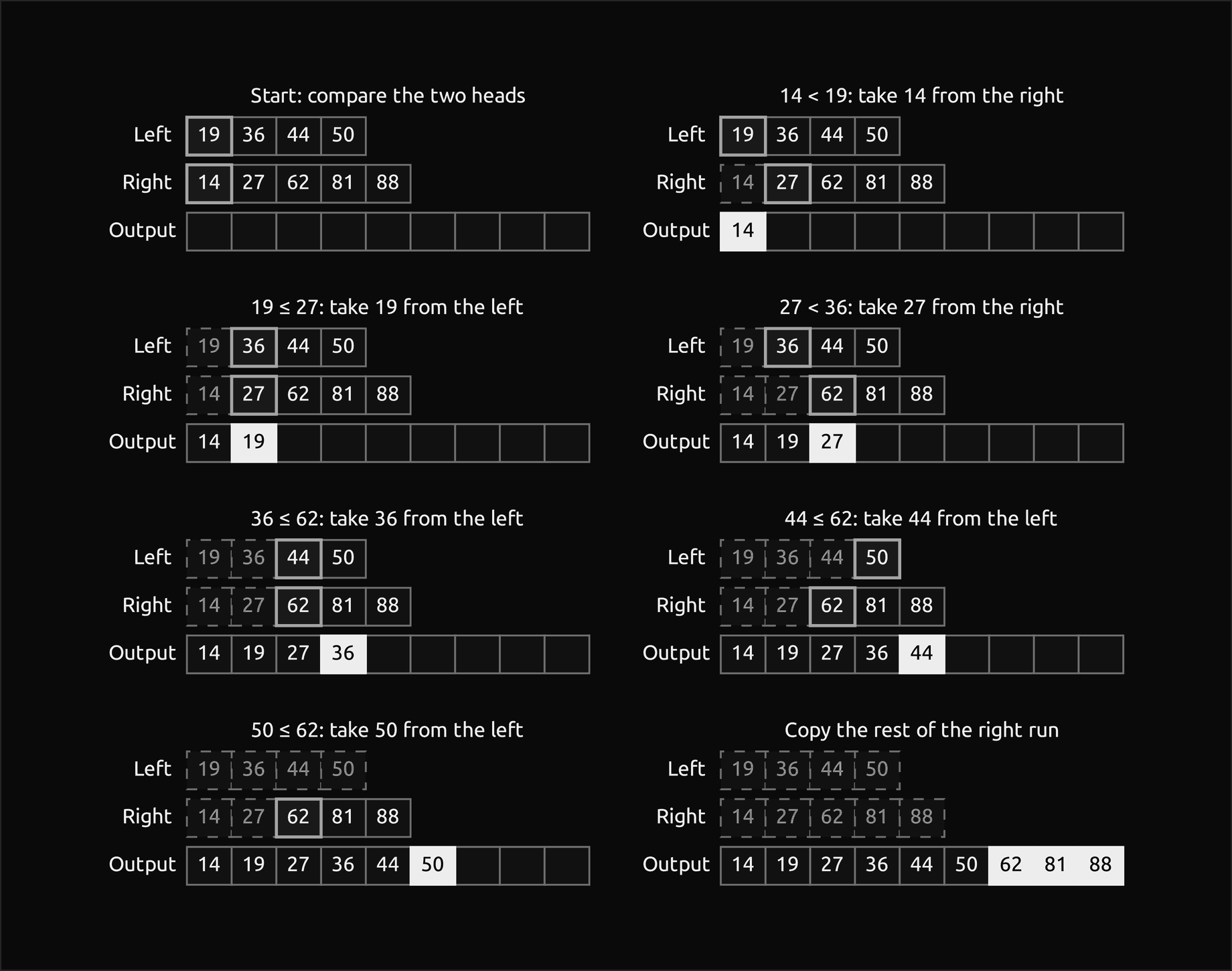
The frames show the heads being compared outlined and the output growing, with its newest items filled. Six comparisons place six items; the last three are copied because the left run is empty, which is why this merge of nine items costs 6 comparisons rather than 8.

Sentinels done correctly

A popular way to write the merge drops the end tests and runs the loop once per output slot: for k from lo to hi − 1, compare the two heads and take the smaller. Written that way the loop is wrong. As soon as one run is used up, its head index points one past the end, and the next comparison reads an item that does not exist: in Python an IndexError, in C whatever memory follows the array. The version is only correct with sentinels.

The sentinel trick copies each run into a new list and closes it with a key larger than every real key, called ∞ here. A used-up run then shows ∞ as its head, ∞ loses every comparison, and the other run's items are taken one comparison each. Three details make it correct:

• The sentinel must be larger than every real key, not merely large. A fixed number such as 1000 or 10^9 fails when real keys can exceed it: merging [40, 2000] with [70] and the sentinel 1000 places the sentinel 1000 and loses the key 2000. Even float("inf") fails when the data contain infinity. The package's TOP is an object whose comparisons say it is larger than anything else, so no real key can tie with it.
• The loop must run exactly hi − lo times, one per real item, and its count, not the sentinels, ends it. The two sentinels never meet, because when both heads would be ∞ every real item has been placed.
• Ties still take the left item, so the sentinel merge is as stable as the merge with end tests.

The price is that a sentinel merge always makes one comparison per item it places, m + n in all, including the comparisons against ∞ that the end tests would have avoided. It also copies both runs out before merging them back. The worked example runs both versions side by side.

Top-down merge sort

Top-down merge sort sorts A[lo:hi] by splitting it at mid = lo + (hi − lo) // 2, sorting A[lo:mid] and A[mid:hi] recursively and merging them. A range of one item is sorted already and returns at once. This split gives the left half ⌊n/2⌋ items and the right half ⌈n/2⌉; the form lo + (hi − lo) // 2 is a habit from languages with fixed-width integers, where lo + hi can overflow, and in Python both forms agree.

Correctness follows by strong induction on the length of the range. A range of length 0 or 1 is sorted. A range of length n ≥ 2 splits into two strictly shorter ranges, which are sorted by the induction hypothesis, and the merge of two sorted runs is sorted. The same argument proves termination: every call works on a shorter range than its caller, so the recursion bottoms out. Splitting into two nonempty halves is essential, and a split that can return the whole range, as the pitfalls show, recurses forever.

The merge writes into A[lo:hi] while it still has to read the two halves, so the halves are first copied into an auxiliary buffer and merged from the buffer back into the array. One buffer of n slots, allocated once before the recursion, serves every merge. The calls form a recursion tree, drawn here for the worked example:

The upper half is the splitting, the middle row the base cases, and the filled lower half the merging, each merge mirrored below its split. Nine items need ⌈log2 9⌉ = 4 levels of splits, and because 9 is not a power of two only one branch, A[7:9], reaches the fourth level. The recursion itself runs depth first: it sorts A[0:4] completely before it touches A[4:9], and the trace in the worked example prints the steps in that order.

Bottom-up merge sort

The recursion only decides which ranges to merge, and those ranges can be listed without it. Bottom-up merge sort treats the input as n runs of one item and makes passes over the array. The pass with width w merges each pair of neighbouring blocks A[lo:lo + w] and A[lo + w:lo + 2w], for lo = 0, 2w, 4w and so on; after it, every block of width 2w is sorted. Widths 1, 2, 4, ... continue until a single run covers the array, which takes ⌈log2 n⌉ passes.

The invariant of the loop is exactly that: before the pass with width w, every block A[lo:lo + w] whose start is a multiple of w is sorted. Two details need care. The last block of a pass can be shorter than w, and when n is not a multiple of 2w the last block may have no partner at all; such a lone block is already sorted and is carried into the next pass unchanged. And the passes must go on while w < n, not only while complete pairs remain, or a short tail is never merged in.

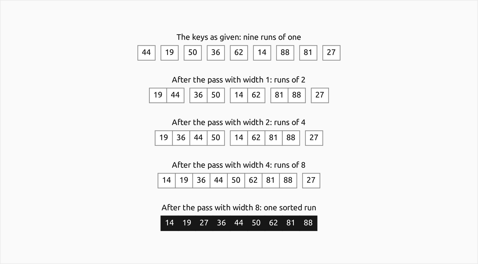
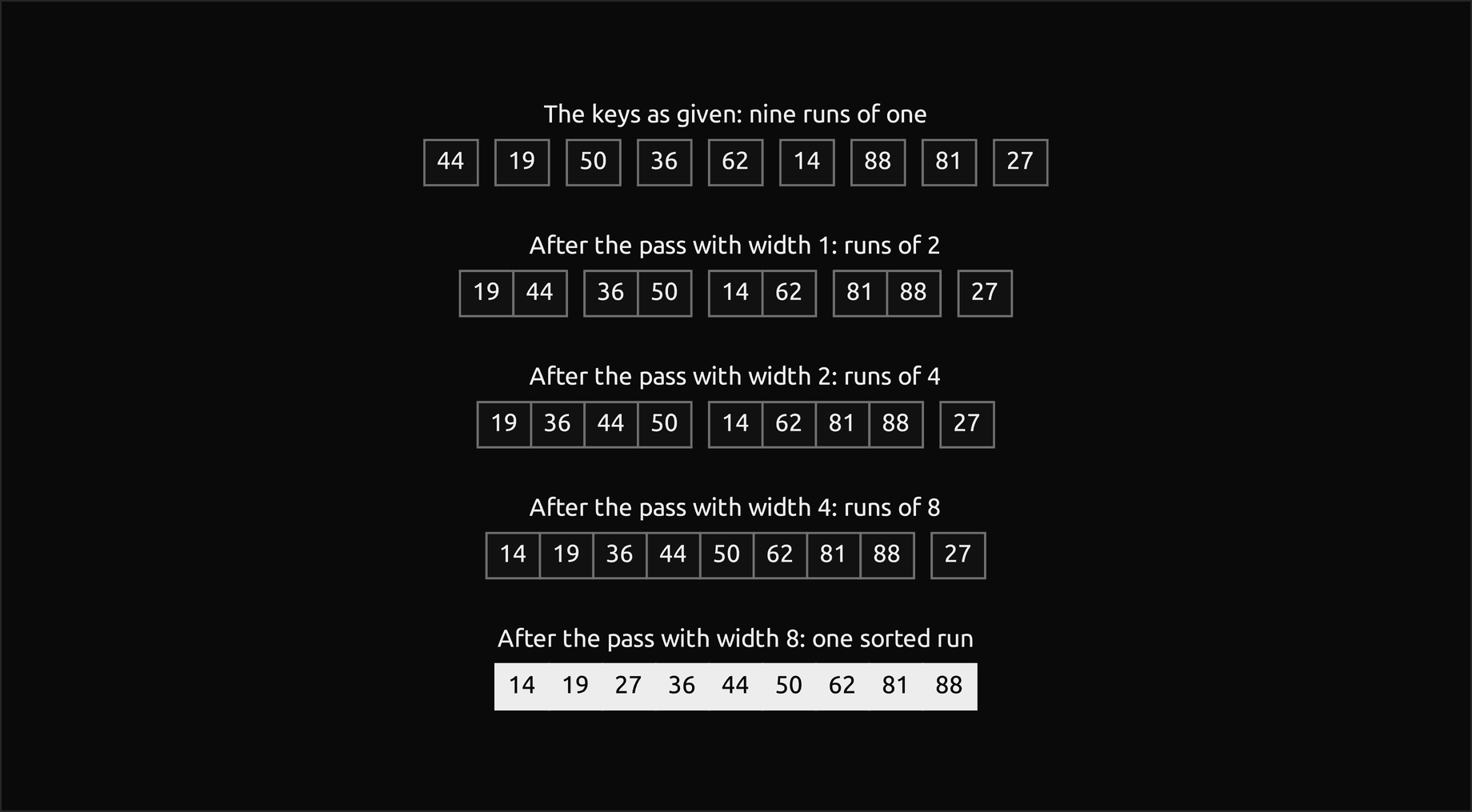
Each row shows the runs after a pass, with a gap between neighbouring runs. The key 27 is carried alone through three passes and only meets the rest in the last merge, of 8 items with 1. For a power of two the bottom-up passes make exactly the merges of the top-down recursion; for other sizes the shapes differ, and so do the counts: 17 comparisons here against 18 top-down.

Without recursion bottom-up merge sort needs no stack at all, and it can merge from one list into the other in each pass instead of copying first, as the next section explains. It is the natural form for linked lists, for external sorting and for parallel sorting, where each pass is a set of independent merges.

Auxiliary space and alternating buffers

Merging two runs in place, inside the array that holds them, is possible but complicated and slower, so practical merge sorts of arrays use an auxiliary buffer of n slots. The recursion of the top-down version adds a stack of about log2 n frames:

The copy-back version moves every item twice per level: once into the buffer and once back. The copy can be avoided altogether by letting the array and the buffer take turns. Start with two equal copies of the input. To sort a range into the target list, sort its two halves into the other list, with the roles swapped, and then merge from the other list into the target. Every merge now reads one list and writes the other, and no copy is needed before it. The precondition that makes this work is that, on entry, the range holds the same items in both lists; the first half's calls touch only their own half, so the second half still meets the precondition when its turn comes, and a range of one item needs nothing because the target already holds it.

Bottom-up merge sort uses the same idea pass by pass: the first pass merges from the array into the buffer, the second from the buffer into the array, and so on. When the number of passes is odd the result ends in the buffer and one final copy brings it back; a function that returns a new list can simply return whichever list holds it. The cost section counts all three ways.

Counting inversions on the way

An inversion is a pair of items in the wrong order:

A sorted array has none and a reversed one has all n(n − 1)/2 of them; insertion sort makes exactly one shift per inversion, which is why it is fast on nearly sorted data. Counting them pair by pair costs Θ(n²) comparisons, but merge sort counts them for free. Any inversion has its two items either in the same half, where the recursive call counts it, or one in each half. A cross pair is never seen by either recursive call, and the merge sees all of them at once: when a right item is taken while items of the left run are still waiting, it overtakes every one of those waiting items, and each of them is larger, so that is mid − i inversions in one step.

Every inversion is counted exactly once, at the one level of the recursion where its two items are first in different halves. Equal items are never counted, because a tie takes the left item. The package's merge_into returns this count, so every sort built on it counts inversions as a by-product.

The count measures how far apart two rankings are. Writing each item of one ranking as its position in the other turns the number of pairs the two rank in opposite order, the Kendall tau distance d, into a count of inversions, and Kendall's rank correlation follows from it:

A tau of 1 means the same order and −1 the reverse order. Recommendation systems, search engines and voting methods compare rankings this way, and the merge-based count is what makes it O(n log n) rather than quadratic.

Natural merge sort and the road to Timsort

Bottom-up merge sort starts from runs of one item, even when the input is nearly sorted. Natural merge sort starts from the runs that are already there. One scan finds them: a run is a maximal stretch that never decreases, or a stretch that strictly decreases, which is reversed in place. The reversal must be limited to strictly decreasing stretches, because reversing a stretch such as 5, 5, 3 would swap the two fives and break stability. The scan compares each pair of neighbours once, n − 1 comparisons, and then neighbouring runs are merged pairwise, pass after pass. Input made of r runs needs ⌈log2 r⌉ passes:

Sorted input is one run and costs n − 1 comparisons, against about (n/2) log2 n for top-down merge sort, and reversed input is one falling run and costs the same. On random input the runs are about two items long and the scan is wasted work.

Timsort, the sort behind Python's sorted and list.sort, is a natural merge sort engineered for real data. It finds runs the same way, reversing strictly falling ones. Runs shorter than a minimum length, minrun, between 32 and 64 and chosen from n, are extended with binary insertion sort, which costs few comparisons on so few items. Runs go on a stack, and merges are chosen by rules on the lengths of the runs at the top, so that merged runs stay balanced and the stack stays short; since Python 3.11 those rules are the powersort policy. And when one run keeps winning during a merge, Timsort switches to galloping, an exponential search for how far that run's lead extends, so that interleaving long blocks costs far fewer than one comparison per item. Sorting in practice takes Timsort apart; this page measures its comparison counts next to the natural merge sort above.

Merge sort on a linked list

A linked list cannot be split in the middle by index arithmetic, but it has a property that makes merge sort fit it better than any other sort: merging two sorted lists needs no buffer. The merge does not move items; it relinks the nodes, setting each chosen node's predecessor to point at it. A dummy node at the front of the output means the first node needs no special case, and when one list runs out, the rest of the other is attached with a single link, because it is already linked in order. Ties take the left node, so the linked merge is stable too.

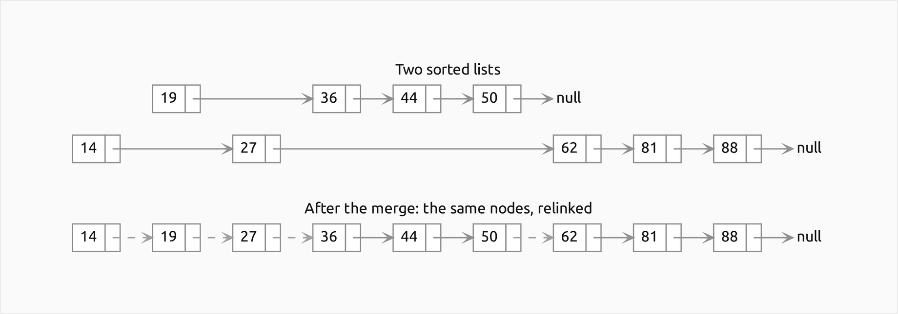
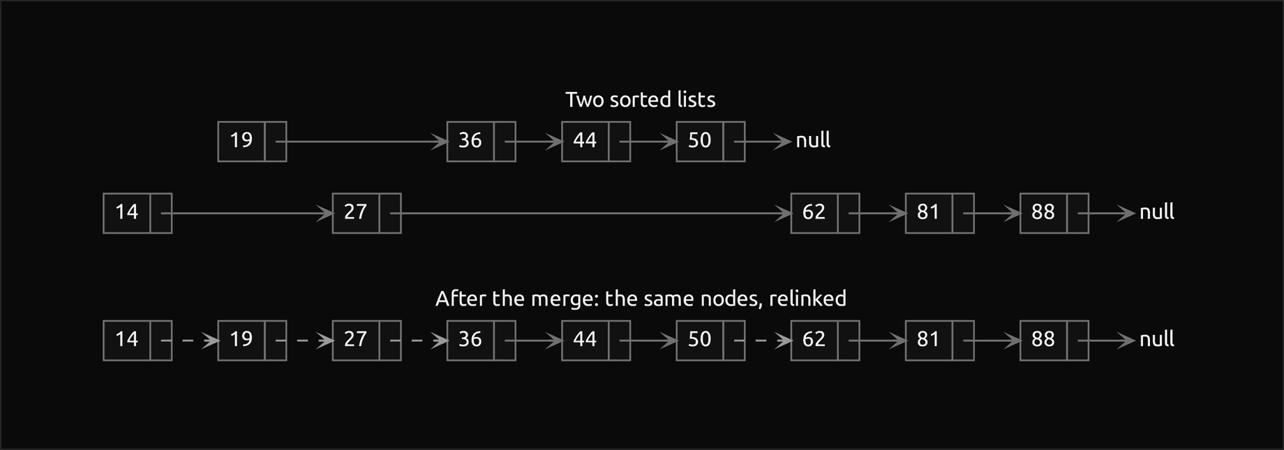
The merged list is made of the same nine nodes. The merge writes 7 next pointers, one per comparison, the first of them in the dummy node, and one to attach the rest; only the 4 dashed ones end up pointing somewhere new, and nothing is copied.

The top-down version counts the list once, cuts it after ⌊n/2⌋ nodes, sorts both halves and merges them; it makes exactly the comparisons of the array version and needs a recursion stack of about log2 n frames. The bottom-up version removes even that. Each pass walks the list, cuts off two runs of the current width, merges them and appends the result to the part already done, and the width doubles after every pass. It holds a dummy node and a few pointers, O(1) extra space, and makes exactly the merges of the array version of bottom-up merge sort. The linked structure itself is the topic of Linked lists.

Merging k runs at once

Merging k sorted runs into one can be done with two-way merges, but how they are arranged matters. Merging the runs one after another into a growing result moves the first run k times, the second k − 1 times and so on. Merging them in rounds, neighbours with neighbours as in bottom-up merge sort, takes ⌈log2 k⌉ rounds and moves every item once per round. A heap does it in one pass: it holds the current head of every run, the smallest head leaves, and the next item of the same run takes its place with one sift-down. The heap here is the BinaryHeap of the heaps topic. Its entries pair each item with its run number and break ties by run number, so that, when the runs are consecutive pieces of one input, equal items leave in input order and the k-way merge is stable.

For the three runs [23, 48, 70], [9, 51, 66, 94] and [31, 35, 57], the heap starts with the heads 23, 9 and 31 and emits 9 first, after which 51 takes its run's place, and so on until 94; the ten items cost 16 comparisons of heap entries, against 13 for two rounds of two-way merges. With so few runs the heap's overhead dominates; its advantage is that it reads every run once, in one pass, which is what an external sort needs. Python's heapq.merge is the same idea and returns the same items in the same order.

External merge sort

When the data are larger than memory, an array sort cannot even start. External merge sort sorts with a fixed budget of M records in memory and files on disk, and it organises the work around passes over the data, because reading and writing files in large sequential blocks costs far more than comparing keys:

• Run formation reads the input M records at a time, sorts each batch in memory and writes it out as a sorted run: ⌈N/M⌉ runs.
• Each merge pass merges the runs k at a time with a heap, reading every run a block at a time. A pass holds k input blocks and one output block in memory, so the block size B is about M/(k + 1). Every pass reads and writes every record once and divides the number of runs by k.

The fan-in k trades memory per block against passes: a larger k means fewer passes but smaller blocks. A different run formation shortens the plan without more memory. Replacement selection keeps a heap of M records ordered by run number and key, writes the smallest record of the current run, and puts the next input record in its place, in the current run if its key is not smaller than the one just written and in the next run otherwise. On random input the runs it writes are about twice as long as memory:

On sorted input replacement selection writes one single run, and only reversed input brings it down to runs of exactly M. Fewer, longer runs can save a whole merge pass.

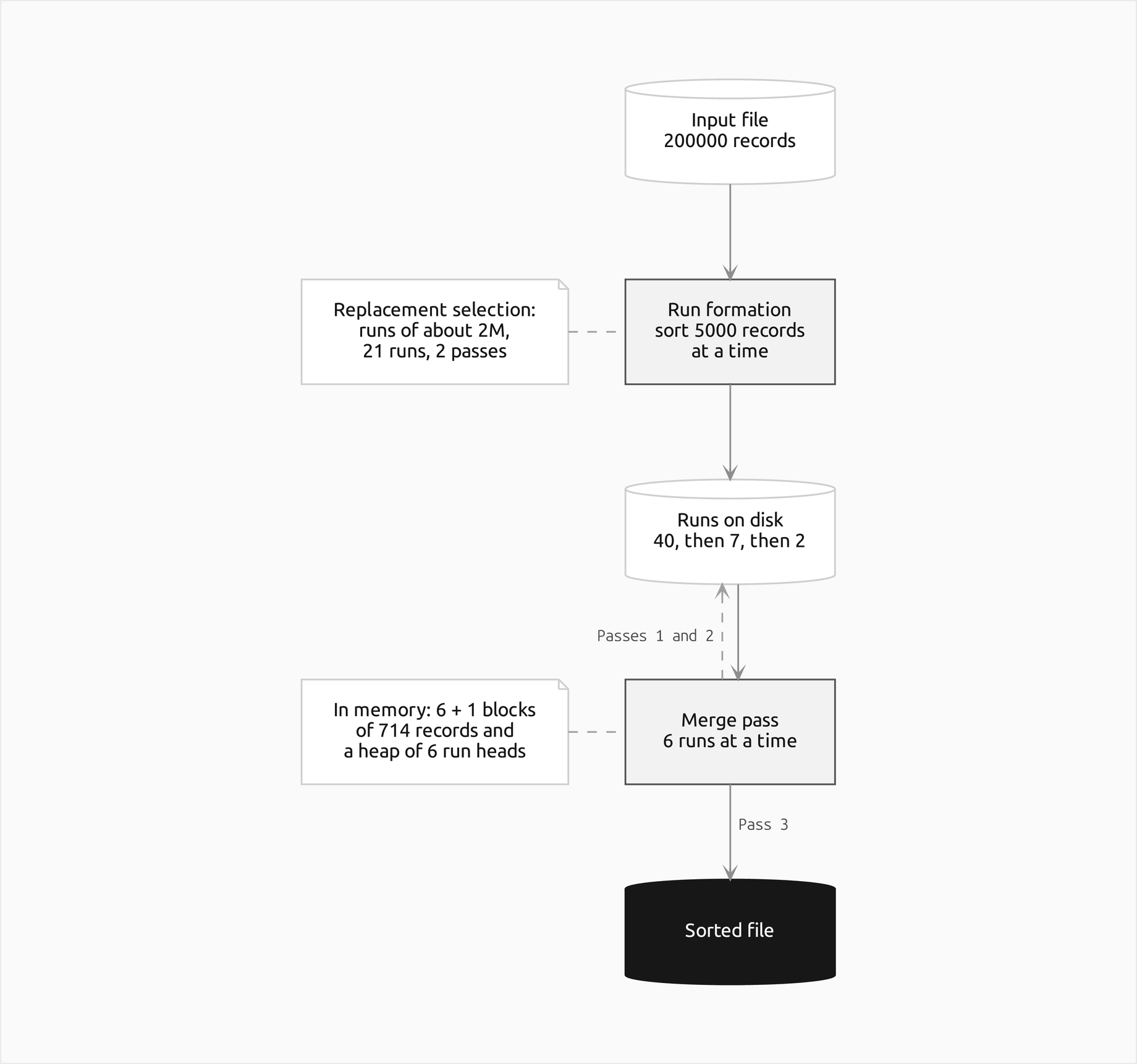
The diagram is the plan of the sample project's default run. Loading and sorting gives 40 runs and needs three merge passes with fan-in 6; replacement selection gives 21 runs, and 21 ≤ 6² means two passes suffice, a quarter less reading and writing. The same reasoning, with blocks of a disk page and fan-ins in the hundreds, is how databases sort for ORDER BY, build indexes and run sort-merge joins, and it is why their tree indexes are the wide B-trees.

Cost

The recurrence and the recursion tree

A call on n items does a constant amount of work to split, makes two recursive calls on the halves and merges in time proportional to n:

The recursion tree solves it. Level d of the tree holds 2^d calls on about n/2^d items each, so the merges of a whole level handle each item at most once and cost at most cn together. For n = 2^h there are h = log2 n levels of merges:

The master theorem of Recurrences gives the same answer, Θ(n log n), as its balanced case. The bound holds for every input, best and worst alike: the splits do not depend on the keys, and every merge of m items costs at least ⌊m/2⌋ comparisons and moves all m items. That is the sense in which merge sort has no bad inputs, unlike quicksort. It does not mean the number of comparisons is the same for all inputs, which the next section makes exact.

Exact comparison counts

Let S(n) be the sizes of all merges added up, the number of items each level merges summed over the levels. It satisfies the recurrence of the sort with cost n per call, and the floors and ceilings can be solved exactly:

In the recursion tree every item is a leaf at depth ⌊log2 n⌋ or ⌈log2 n⌉, and S(n) is the sum of those depths; the closed form counts the 2(n − 2^⌊log2 n⌋) leaves on the deeper level once more. For the nine worked keys S(9) = 9·3 + 2·1 = 29.

The worst case W(n) charges every merge its maximum, its size minus one. There are n − 1 merges, one per internal node of the tree, so:

The bound is reached. To make a merge cost its size minus one, the last two items must come from different runs, and the simplest way is to let the two runs alternate in sorted order. Undoing the merges gives the worst input: put the items at odd positions of the sorted order in the left half and those at even positions in the right half, and arrange each half the same way. For eight keys 0 to 7 this gives [7, 3, 5, 1, 6, 2, 4, 0], which costs W(8) = 17 comparisons, and the package's worst_case_input reaches W(n) exactly for every n tested.

The best case B(n) charges every merge only its left half, which is the shorter one with this split. Sorted input achieves it, because every left run is used up before the right run wins once:

Here ν(k) is the number of ones in the binary form of k, so B(n) is the number of one bits written out when counting from 0 to n − 1, about (n/2) log2 n. For n = 9, B(9) = 13. The comparisons of every input lie between B(n) and W(n), and the merge with sentinels, which compares once per item placed, always makes the largest number of all:

The leading term of W(n) is n log2 n; the term that follows wobbles. Writing θ for the distance from log2 n up to the next integer:

So W(n) is n log2 n minus between 0.91n and n, plus one. No comparison sort can do much better in the worst case: it has to tell n! orders apart with yes or no answers, which needs log2 n! comparisons, a bound derived in The sorting lower bound and linear-time sorts:

Merge sort's worst case exceeds the lower bound by less than 0.53n comparisons. On random permutations it averages about n log2 n − 1.26n, between the two.

Counted comparisons

The example comparison_counts.py counts the comparisons of merge_sort on sorted input, on the constructed worst-case input and on five random permutations per size, for n from 2 to 1024.

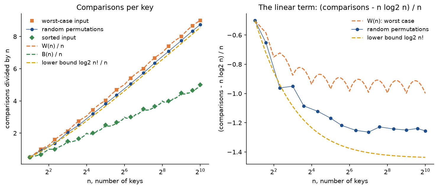
Per key, n log2 n is a straight line on this axis. On the left, the measured best and worst cases sit exactly on their predictions at every size tested, and random input lies close to the worst case: at n = 1024 the counts are B = 5120, a random mean of 8953.8, W = 9217 and a lower bound of 8769.0, with the sentinel count S = 10240 above them all. The right panel subtracts the leading term. The worst case traces the wave of the formula above, and at n = 16384 random permutations average (C − n log2 n)/n = −1.2595 against −1.4422 for the lower bound and −0.9999 for the worst case, which is −1 + 1/n exactly at a power of two.

Space and data movement

Comparisons are not the whole cost; every merge also moves items. Counting a move as one write of an item into an array slot:

The example space_and_moves.py counts moves for the three array versions and pointer writes, called links, for the bottom-up linked-list sort.

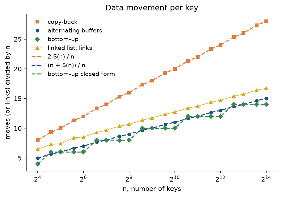
Every array count equals its closed form. Alternating buffers halve the data movement: at n = 16384 the copy-back version moves 28 items per key, 2 log2 n, the alternating version 15 and bottom-up 14. Bottom-up moves in steps, because an extra pass is needed only when n passes a power of two, and an odd number of passes costs one copy back. The linked list moves no items at all and writes 16.7 links per key: one per comparison, plus a few for every merge and every cut.

Memory tells the same story. Measured with tracemalloc while sorting 50000 keys, a list of that many references takes about 390.6 KiB. The top-down sort that returns a new list peaks at about 1563 KiB: the result, the buffer and temporaries that Python's slice copying makes. Bottom-up sorting in place needs one buffer, 404 KiB. Both linked-list sorts allocate under 1 KiB, the top-down one because its recursion is only 17 calls deep and the bottom-up one because it holds a dummy node and a few pointers; their price is paid earlier, in the next pointer every node carries.

Small blocks: the cutoff

Recursing all the way down to single items spends most calls on tiny ranges: a full recursion makes 2n − 1 calls, half of them on single items. Library merge sorts stop splitting at blocks of some small size k and sort those by insertion sort. The cost has two parts, the blocks and the merges above them:

The first part grows with k and the second shrinks, so k must stay small: any k up to about log n keeps the total at Θ(n log n). The example measures it on 4096 random keys:

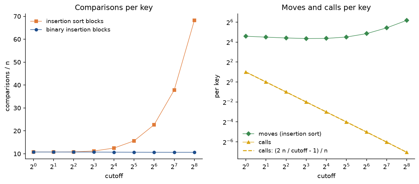
Calls fall in proportion to the cutoff, from 1.9998 per key to 0.2498 at cutoff 8. Comparisons barely move at first, 10.7537 per key without a cutoff and 11.1992 at cutoff 8, and moves even fall, from 24 to 20.4502 per key, because a block sorted in place needs no buffer copy. Beyond 16 the quadratic block sort takes over. Binary insertion sort keeps comparisons flat, 10.6394 per key even at cutoff 256, but it still shifts items one slot at a time, so its moves grow just the same. In C or Python, where a call and a buffer copy cost more than a comparison, cutoffs between about 8 and 64 pay off; that is the range of Timsort's minrun.

Runs, k-way merging and other cost variants

The example runs_and_kway.py sorts 4096 keys made of r ascending runs, for r from 1 to about 1000, and random keys.

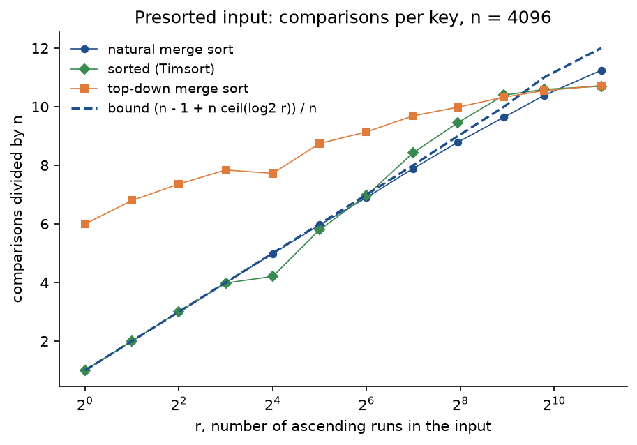
Natural merge sort follows its bound, n − 1 comparisons for one run, 3.9958 per key for 8 runs and 6.8994 for 64, and sorted tracks it, while top-down merge sort spends 6 per key even on sorted input, (n/2) log2 n. On random input, with runs about two keys long, the scan for runs is wasted and natural merge sort needs 11.2422 per key against 10.7217 for top-down; Timsort avoids this loss by extending short runs to minrun with binary insertion sort.

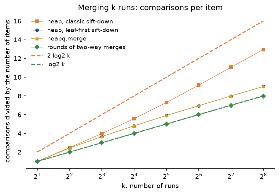
All the k-way methods grow like log2 k per item. Rounds of two-way merges are the cheapest in comparisons, 7.9662 per item for 256 runs; the heap with the leaf-first sift-down, which heapq.merge also uses, needs one more, 9.0085, and the classic sift-down, two comparisons per level, 12.9511. Merging the 256 runs one after another needs 123.7942 comparisons per item. The heap's extra comparison buys the property that matters for files: one pass, every run read once, in sequence.

The bounds of the k-way merge hold for any shape of input. With many short runs the order of the merges decides the cost: for 128 runs of 128 items, 16384 in all, seven rounds of two-way merges cost 114441 comparisons and exactly 114688 moves, (n/2) log2 n, while merging the runs one after another costs 1048328 comparisons and 1056768 moves, n(k + 1)/2, more than nine times as much.

The other cost that can change is the comparison itself. Every count on this page assumes that comparing two keys costs one step, which holds for numbers but not for strings:

A comparison of two strings reads their common prefix and one more character, so strings that share long prefixes make every comparison expensive. Sorting strings of length 48 that share their first 44 characters read 45.2313 characters per comparison for 64 strings and 45.7555 for 4096, where 43967 comparisons read 2011734 characters: the comparison count grows like n log2 n, and every comparison costs about the length of the shared prefix. Radix sorts and string-specific merge sorts that remember common prefixes avoid this.

Worked example

Every step below is printed by examples/worked_example.py and asserted by tests/test_worked_example.py. The keys are the nine integers 44, 19, 50, 36, 62, 14, 88, 81 and 27.

Splitting and merging nine keys

Top-down merge sort splits A[lo:hi] at lo + (hi − lo) // 2, so the left half is the shorter one. Level by level, the splits are:

• Level 0: A[0:9] splits into A[0:4] = [44, 19, 50, 36] and A[4:9] = [62, 14, 88, 81, 27].
• Level 1: A[0:4] into [44, 19] and [50, 36]; A[4:9] into [62, 14] and [88, 81, 27].
• Level 2: each pair into its two single keys; [88, 81, 27] into [88] and [81, 27].
• Level 3: [81, 27] into [81] and [27].

The merges then run from the deepest level up, each with its comparisons:

• [81] and [27] give [27, 81]: 1 comparison.
• [44] and [19] give [19, 44], [50] and [36] give [36, 50], and [62] and [14] give [14, 62]: 1 comparison each.
• [88] and [27, 81] give [27, 81, 88]: 27 < 88 and 81 < 88, then 88 is copied; 2 comparisons.
• [19, 44] and [36, 50] give [19, 36, 44, 50]: 19 ≤ 36, 36 < 44, 44 ≤ 50, then 50 is copied; 3 comparisons.
• [14, 62] and [27, 81, 88] give [14, 27, 62, 81, 88]: 14 ≤ 27, 27 < 62, 62 ≤ 81, then 81 and 88 are copied; 3 comparisons.
• [19, 36, 44, 50] and [14, 27, 62, 81, 88] give [14, 19, 27, 36, 44, 50, 62, 81, 88]: 6 comparisons, traced below.

The recursion makes these merges in a different order, depth first: it finishes [19, 36, 44, 50] before it splits A[4:9]. The whole sort costs 18 comparisons, 58 moves (2 S(9) = 2 · 29, since each merged item is copied into the buffer and back) and 17 calls, at most 5 deep. The comparisons lie between the best case B(9) = 13 and the worst case W(9) = 21; the sentinel version would make S(9) = 29.

The last merge, one comparison at a time

The final merge joins L = [19, 36, 44, 50] and R = [14, 27, 62, 81, 88]:

• 19 against 14: 14 < 19, take 14 from the right.
• 19 against 27: 19 ≤ 27, take 19 from the left.
• 36 against 27: 27 < 36, take 27 from the right.
• 36 against 62: 36 ≤ 62, take 36 from the left.
• 44 against 62: 44 ≤ 62, take 44 from the left.
• 50 against 62: 50 ≤ 62, take 50 from the left.
• The left run is used up, so 62, 81 and 88 are copied from the right without comparisons.

Six comparisons and nine moves. The merge stops two comparisons short of the maximum of 8 because 81 and 88, the two largest keys, are both in the right run.

The same merge with sentinels

The sentinel version copies the runs into [19, 36, 44, 50, ∞] and [14, 27, 62, 81, 88, ∞] and runs its loop exactly nine times. The first six comparisons are those above. Then the left head is ∞:

• ∞ against 62: 62 < ∞, take 62.
• ∞ against 81: 81 < ∞, take 81.
• ∞ against 88: 88 < ∞, take 88.

The loop has placed nine items and stops; the two sentinels never meet. Nine comparisons, one per item, and 18 moves: nine to copy the runs out and nine to write them back.

Bottom-up passes

Bottom-up merge sort of the same keys makes four passes:

• Width 1: merges 44 and 19, 50 and 36, 62 and 14, 88 and 81, one comparison each, and carries 27: [19, 44 | 36, 50 | 14, 62 | 81, 88 | 27], 4 comparisons.
• Width 2: merges [19, 44] with [36, 50] in 3 comparisons and [14, 62] with [81, 88] in 2, and carries 27: [19, 36, 44, 50 | 14, 62, 81, 88 | 27], 5 comparisons.
• Width 4: merges the two runs of four, 14 < 19 and then 19, 36, 44 and 50 each before 62, and carries 27: [14, 19, 36, 44, 50, 62, 81, 88 | 27], 5 comparisons.
• Width 8: merges the run of eight with [27]: 14 ≤ 27, 19 ≤ 27, 27 < 36, then the left run's remaining six keys are copied: 3 comparisons.

In all 17 comparisons and 36 moves: four passes of nine moves, and since four is even the result is already back in the array. The passes merge different ranges from the top-down recursion, a final merge of 8 with 1 instead of 4 with 5, which is why the count differs.

Inversions on the way

The nine keys hold 15 inversions: (44, 19), (44, 36), (44, 14), (44, 27), (19, 14), (50, 36), (50, 14), (50, 27), (36, 14), (36, 27), (62, 14), (62, 27), (88, 81), (88, 27) and (81, 27). The top-down merges find them:

• Each of the four merges of two single keys finds 1, because in each pair the left key is larger.
• [88] with [27, 81] finds 2: 27 overtakes 88, then 81 overtakes 88.
• [19, 44] with [36, 50] finds 1: 36 overtakes the waiting 44.
• [14, 62] with [27, 81, 88] finds 1: 27 overtakes the waiting 62.
• The final merge finds 7: 14 is taken while all four left keys wait, 4 inversions, and 27 while 36, 44 and 50 wait, 3 more.

That is 4 + 2 + 1 + 1 + 7 = 15, at no extra comparison. Insertion sort on the same keys would shift items exactly 15 times.

Natural runs

Natural merge sort of [12, 25, 61, 7, 33, 40, 58, 94, 21, 18, 3] first scans for runs with 10 comparisons, one per pair of neighbours, and finds three: [12, 25, 61], [7, 33, 40, 58, 94] and the falling [21, 18, 3], which it reverses to [3, 18, 21]. The first pass merges the first two runs into [7, 12, 25, 33, 40, 58, 61, 94] in 7 comparisons and carries [3, 18, 21]; the second pass merges those two in 5 comparisons. The sort costs 22 comparisons and 25 moves, three of them for the reversal.

The code

The package merge_sort is plain Python, one idea per module. Importing it needs only the standard library and the heaps_and_priority_queues package of the heaps topic, which kway.py and the project use for their heap; Matplotlib is imported by plotting.py alone and SciPy inside scipy_kendall_tau.

• merging.py holds merge_into, the merge with explicit run ends on which every array sort is built, merge for two lists and merge_comparison_range. merge_into returns the inversions between its runs.
• sentinels.py holds TOP, a key larger than every other key, merge_with_sentinels and sentinel_merge_sort.
• top_down.py holds split_point, merge_sort and sort_range, the copy-back recursion; buffers.py holds merge_sort_alternating and sort_into, the version with alternating buffers.
• bottom_up.py holds bottom_up_sort, which sorts in place with ping-pong buffers, bottom_up_merge_sort and bottom_up_passes.
• recursion_tree.py records the calls of top-down merge sort as CallNode objects for traces and drawings: recursion_tree, tree_levels and merges_by_level.
• hybrid.py holds merge_sort_with_cutoff with straight and binary insertion sort for small ranges.
• natural.py holds find_runs, count_runs, natural_merge_sort and natural_passes.
• inversions.py holds sort_and_count, count_inversions, the brute-force reference, kendall_tau_distance and kendall_tau.
• linked_lists.py holds the Node class and cut; linked_sort.py holds merge_linked, linked_merge_sort and linked_bottom_up_sort.
• kway.py holds kway_merge, a lazy heap merge of any number of iterables, and pairwise_merge and sequential_merge for comparison.
• bounds.py holds every closed form of the cost section, the recurrences they solve, and worst_case_input, which builds the inputs that reach W(n).
• counting.py holds OperationCounter, with the fields comparisons, moves, links and calls, CountedKey, which counts the comparisons of library code, and CharacterKey, which counts the characters a string comparison reads.
• trace.py holds the Step record and format_trace, which prints splits, comparisons, copied remainders, merges and passes. drawing.py returns the Graphviz text of arrays cut into runs (Frame and frames_dot, with array_dot and before_after_dot for one or two states) and of the recursion tree, with every node pinned at a position the code computes; tree_layout.py holds the tidy layout that places the recursion tree, pinned.py the style, sizes and cell roles every drawing shares, merge_frames.py draws one merge frame by frame and linked_drawing.py the linked merge.
• invariants.py holds sorted_violation, is_sorted, check_sorted, stability_violation, check_sort_result and the checks of the merge's loop invariant, the pass invariant and linked lists.
• workloads.py holds the worked example's keys and seeded inputs; comparisons.py puts sorted, heapq.merge and SciPy next to the package; pitfalls.py holds deliberately broken versions for the pitfalls below; plotting.py draws every plot in the handbook's colours.

Counting and tracing never change what the code does. Every sort accepts an optional counter and an optional trace list, and the trace of the merge records each comparison with the two heads and the side it took, which is all format_trace needs to print the lines of the worked example.

The examples run in a few seconds each from the repository root:

• examples/worked_example.py prints every step of the worked example and writes the three generated diagram sources of the merge, the recursion tree and the bottom-up passes.
• examples/comparison_counts.py measures best, worst and random comparison counts against the closed forms and counts the characters read when sorting strings.
• examples/space_and_moves.py measures moves, links and memory, and the effect of a cutoff, and writes the linked-merge diagram source.
• examples/runs_and_kway.py measures natural merge sort on presorted input and the four ways of merging k runs.
• examples/common_mistakes.py runs every broken version from pitfalls.py next to the correct code.
• examples/compare_with_sorted.py checks every sort against sorted, counts the comparisons of Timsort on several inputs, checks heapq.merge and Kendall's tau, and times one sort.
• examples/practice.py prints fresh exercises with their solutions; --seed gives a new set.

python searching-and-sorting/merge-sort/examples/worked_example.py
python searching-and-sorting/merge-sort/examples/comparison_counts.py
python searching-and-sorting/merge-sort/examples/space_and_moves.py
python searching-and-sorting/merge-sort/examples/runs_and_kway.py
python searching-and-sorting/merge-sort/examples/common_mistakes.py
python searching-and-sorting/merge-sort/examples/compare_with_sorted.py
python searching-and-sorting/merge-sort/examples/practice.py --seed 7

The sample project, project/external_sort.py with its helpers project/record_files.py, project/run_formation.py and project/merge_passes.py, sorts a text file of records that is larger than its memory budget. Each record is one line with a four-letter random key, a serial number and a payload, so equal keys are common and the serial numbers show whether ties keep their input order. The program never holds more than the budget of M records plus one block in memory: run formation either loads and sorts M records at a time with the package's merge_sort or uses replacement selection on the heaps topic's BinaryHeap, and the merge passes merge k runs at a time with the package's kway_merge, reading and writing every file a block of about M/(k + 1) records at a time. It counts records and blocks read and written and every comparison, and checks every output line by line against sorting the whole file in memory with sorted. The default run sorts 200000 records with memory for 5000 and fan-in 6 by both methods, shows replacement selection on random, sorted and reversed input, and sweeps the fan-in from 2 to 16 on 40000 records with memory for 1000. All files live in a temporary directory that is removed at the end, and the run takes about 10 seconds. Options --records, --memory, --fan-in, --sweep, --sweep-records, --sweep-memory and --seed change the setup, and --figures writes the PNG elsewhere.

python searching-and-sorting/merge-sort/project/external_sort.py
python searching-and-sorting/merge-sort/project/external_sort.py --records 500000 --memory 2000 --fan-in 16

In the default run, loading and sorting writes 40 runs of exactly 5000 records and needs 3 merge passes, so it reads and writes 800000 records each, 2N(1 + 3); replacement selection writes 21 runs averaging 1.9048 M and needs only 2 passes, 600000 reads and 600000 writes. Both outputs equal the in-memory sort, ties included. On 20000 records with memory for 1000, replacement selection writes 11 runs averaging 1.8182 M on random input, one run on sorted input and 20 runs of exactly M on reversed input.

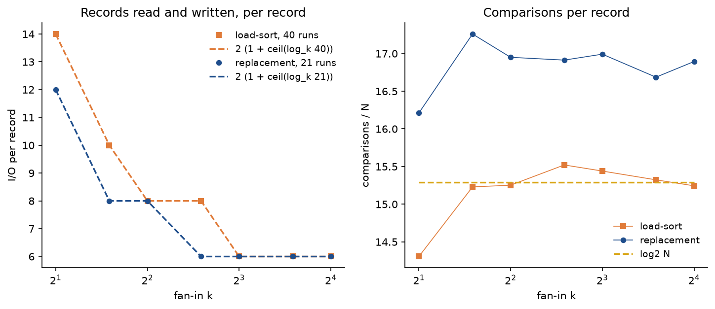
The reads and writes fall in steps, one step for every pass the larger fan-in saves, and they match the plan exactly. The comparisons hardly depend on k: whatever the plan, sorting N records by comparisons costs about N log2 N of them, 15.3 per record here, and only the reading and writing changes. Replacement selection makes about 1.5 more comparisons per record, the price of its heap, and saves a pass at fan-ins 2, 3 and 6.

The notebook merge_sort.ipynb follows this page: the merge and its invariant, the worked example, the diagrams, the exact counts, inversions, natural runs, linked lists, the k-way merge and a small external sort. The tests in tests check the worked example value by value, the merge's loop invariant after every comparison of hundreds of random merges, the pass invariant, stability on thousands of records with repeated keys, every closed form against counted operations and the agreement with sorted, heapq.merge and SciPy, and run in a few seconds:

python -m pytest searching-and-sorting/merge-sort

All data are synthetic, generated from seeds by workloads.py and project/record_files.py, so nothing is downloaded and no licence is involved.

In practice

Python's sorted and list.sort

Python's sorted and list.sort run Timsort, a natural merge sort written in C. Like every sort in the package they are stable and compare items with < only, so on any input they return the same items in the same order, ties included; examples/compare_with_sorted.py checks this on 5000 records with repeated keys for six versions of the package:

from merge_sort import bottom_up_merge_sort, merge_sort, random_records

records = random_records(5000, seed=2, spread=20)
expected = [id(record) for record in sorted(records)]
assert [id(record) for record in merge_sort(records)] == expected
assert [id(record) for record in bottom_up_merge_sort(records)] == expected

Counted through wrapped keys on 4096 keys, sorted makes 43847 comparisons on a random permutation against 43897 for merge_sort, and 4095 on sorted or reversed input, where top-down merge sort spends 24576. Two interleaved sorted halves cost it 8190 comparisons, one scan and one merge, so sorted(a + b) is a perfectly good way to merge two sorted lists in Python. In wall-clock time sorted is about 24 times faster than the package's merge_sort on 100000 integers, the usual gap between C and Python.

Stability is what makes sorting by several keys simple: sort by the minor key first and then by the major key, and the second sort keeps the first order among ties. Usually a single sort with a key function that returns a tuple does the same in one pass. The key function is called once per item, and the results are cached for the sort, which is cheaper than comparing through functools.cmp_to_key.

heapq.merge and merging files

heapq.merge(*iterables) merges sorted inputs lazily with a heap of one entry per input, exactly as kway_merge does, and returns the same items: merging 16 runs of 6340 items in total, it made 30447 comparisons against 30498 for the package. It reads one item ahead per input, so it can merge files, generators and network streams far larger than memory, and it accepts key and reverse arguments. When to use which:

• Use sorted or list.sort for anything that fits in memory; they are stable, adaptive to runs and fast.
• Use sorted(a + b) to merge two sorted lists that fit in memory, and heapq.merge when the inputs are streams or many, or too large to concatenate.
• Use an external merge sort, or a tool that implements one, when the data do not fit in memory: the Unix sort command does, writing sorted runs to temporary files and merging them, and so does every database.
• Use the merge-based inversion count for rank distances; scipy.stats.kendalltau gives Kendall's tau directly and agreed with kendall_tau to 0.6898 on two rankings of 50 items 190 pairs apart.
• Use merge sort itself on linked lists, where it needs no buffer and every other good sort needs random access.

Elsewhere

Java sorts arrays of objects and all List.sort calls with Timsort, because the sort must be stable, and arrays of primitives with a dual-pivot quicksort, where stability cannot be observed. C++'s std::stable_sort is a merge sort that uses a buffer when it can get one and falls back to merging in place, in O(n log² n), when it cannot; std::list::sort is a merge sort on the list's nodes. Rust's stable slice::sort is a merge sort as well, and Go's sort.Stable sorts blocks by insertion and merges them in place with rotations. Merge sort parallelises naturally, since the two halves are independent and the merges of one pass are too, which is why GPU and multi-core sorting libraries and the sort phase of MapReduce frameworks are built on merging. Databases use external merge sorts for ORDER BY, index builds and sort-merge joins, and log-structured storage engines merge sorted files continually in their compactions. The fastest sorts of integers and short strings are radix sorts, which beat any comparison sort once the keys are fixed-width; Quicksort wins in place on arrays when stability is not needed.

Pitfalls

• Merging without end tests or sentinels. A loop that runs once per output slot and compares the two heads reads past the end of a run as soon as one is used up; in Python it raises IndexError, in C it reads garbage. Either test both ends, i < mid and j < hi, or close both runs with sentinels. examples/common_mistakes.py runs this and every following mistake.
• A sentinel that a real key can reach. With 1000 as the sentinel, merging [40, 2000] with [70] gives [40, 70, 1000]: the sentinel is placed as an item and 2000 is lost. Use a value that compares larger than every key, such as the package's TOP, or explicit end tests.
• Forgetting the rest of a run. A merge that stops when either run is empty and does not copy the rest of the other loses items: [19, 36, 44, 50] and [14, 27, 62, 81, 88] give only six of their nine keys.
• Taking the right item on ties. The output is still sorted, but equal keys from the right run overtake those from the left, so the sort is no longer stable. Take the right item only when it is strictly smaller.
• Mixing inclusive and exclusive ends. Splitting an inclusive range [lo, hi] into [lo, mid − 1] and [mid, hi] makes no progress on two items, since mid = lo, and recurses forever. Pick half-open ranges and split at lo + (hi − lo) // 2 into [lo, mid) and [mid, hi), and check that both halves are nonempty for every range of two or more items.
• Stopping bottom-up passes too early. Passes that merge only complete pairs of blocks never merge the tail when n is not a power of two: the worked keys come out as [14, 19, 36, 44, 50, 62, 81, 88, 27]. Run passes while the width is below n, merge a short last block and carry a lone one.
• Returning the wrong buffer. With alternating buffers, the result is in the buffer after an odd number of passes. Returning the original list then returns the state of the previous pass: [61, 17, 45, 8, 33, 29] comes back as [8, 17, 45, 61, 29, 33].
• Counting one inversion per right item taken. A right item overtakes every left item still waiting, mid − i of them; counting one gives 10 instead of 15 for the worked keys. Counting ties as inversions, by taking the right item on ties, gives 3 instead of 2 for [2, 2, 1].
• Splitting a linked list with the fast pointer at the head. With slow and fast pointers that both start at the head, a list of two nodes splits into two nodes and none, and the recursion never ends. Start the fast pointer at head.next, or count the nodes and cut after half of them.
• Reversing falling runs that contain equal keys. Natural merge sort may reverse a falling run only when it falls strictly; reversing 5a, 5b, 3c gives 3c, 5b, 5a and breaks stability.
• Believing that merge sort has no worst case. Its running time is Θ(n log n) on every input, but its comparison count varies from B(n) to W(n), 13 to 21 for nine keys, and the worst input can be built. When hand-tracing, count comparisons merge by merge, and remember that a merge stops comparing as soon as one run is empty.
• Choosing the cutoff from the merge term alone. The merges above blocks of k items cost about n log2(n/k), which only falls as k grows, while insertion sort on the blocks costs Θ(nk), which grows; on 4096 random keys the moves are lowest at cutoffs 8 and 16 and more than three times higher at 256. Pick k from both terms, or measure it.
• Writing a trace that hides the structure. A hand trace that lists only the final array, or mixes the levels, cannot be checked. Write the splits level by level, then each merge with its two input runs, its result and its comparisons, as the worked example does.

Further reading

• D. E. Knuth, The Art of Computer Programming, volume 3, Sorting and Searching, second edition, sections 5.2.4 and 5.4, Addison-Wesley, 1998. Merging, merge sort and its exact analysis, replacement selection and external sorting.
• T. H. Cormen, C. E. Leiserson, R. L. Rivest and C. Stein, Introduction to Algorithms, fourth edition, section 2.3 and chapter 4, MIT Press, 2022. Merge sort, its correctness and its recurrence; the third edition writes the merge with sentinels.
• R. Sedgewick and K. Wayne, Algorithms, fourth edition, section 2.2, Addison-Wesley, 2011. Top-down and bottom-up merge sort, the cutoff to insertion sort and eliminating the copy to the auxiliary array.
• J. Kleinberg and É. Tardos, Algorithm Design, section 5.3, Pearson, 2005. Counting inversions by merge sort.
• P. Flajolet and M. Golin, "Mellin transforms and asymptotics: the mergesort recurrence", Acta Informatica 31(7), 673-696, 1994. The oscillating terms in the best, average and worst cases.
• W. Panny and H. Prodinger, "Bottom-up mergesort: a detailed analysis", Algorithmica 14(4), 340-354, 1995.
• T. Peters, listsort.txt in the CPython source tree. The design of Timsort: runs, minrun, the merge stack and galloping.
• J. I. Munro and S. Wild, "Nearly-optimal mergesorts: fast, practical sorting methods that optimally adapt to existing runs", Proceedings of ESA, 63:1-63:16, 2018. Powersort, the merge policy of CPython since 3.11.
• N. Auger, V. Jugé, C. Nicaud and C. Pivoteau, "On the worst-case complexity of TimSort", Proceedings of ESA, 4:1-4:13, 2018.
• A. Aggarwal and J. S. Vitter, "The input/output complexity of sorting and related problems", Communications of the ACM 31(9), 1116-1127, 1988. Why multiway merging is optimal for data on disk.
• M. G. Kendall, "A new measure of rank correlation", Biometrika 30(1/2), 81-93, 1938.
• The Python documentation: the Sorting HOW TO, and the heapq module's merge.