Breadth-first and depth-first search¶

Almost every question about a graph starts by visiting its vertices in a systematic way: which vertices can be reached from here, how many steps away is each one, is there a cycle, can the vertices be split into two sides, in which order may these tasks run. Breadth-first search (BFS) and depth-first search (DFS) are the two systematic ways, and both visit every reachable vertex and look at every edge exactly once, in time proportional to the size of the graph. They differ in the order of their visits, and that order is what makes each one useful: BFS moves outwards in layers and finds paths with the fewest edges, while DFS follows one path as deep as it goes, and the times at which it enters and leaves each vertex expose the structure of the graph. This page builds a small adjacency-list graph, derives BFS with its layers, parent tree and fewest-edge paths and proves them right, tests bipartiteness, develops recursive DFS with discovery and finish times, the parenthesis structure, the white-path theorem, the four classes of edges and cycle detection, rewrites DFS without recursion, and shows why the popular stack search that marks vertices as it pushes them is not a depth-first search at all. Afterwards you will be able to trace either search by hand, queue by queue and time by time, implement both for explicit and implicit graphs, and know when a fewest-edge path is not the answer. It builds on Stacks, Queues and deques and Recursion, and it is the base of Topological sorting, Connected components and Single-source shortest paths.

The traversals need only the standard library; to run the plots and the notebook install the base group, and the graphs group for the comparisons with NetworkX and SciPy. The sample project downloads one public-domain word list on its first run.

Intuition¶

Drop a stone into a still pond. The ripple reaches every point at distance one before any point at distance two, and the order in which it arrives at things is the order of their distance from the stone. Breadth-first search is that ripple on a graph: it first visits every neighbour of the start, then every vertex two edges away, then three, so when it first reaches a vertex it has done so along a path with as few edges as possible.

Now explore a cave with a ball of thread tied to the entrance. You walk down a passage as far as it goes, and when you reach a dead end, or a chamber you have seen before, you wind the thread back to the last junction with an unexplored passage and try that one. You are never far from a way back, and the thread itself, the path from the entrance to where you stand, is all you need to remember. Depth-first search is that walk. Its order says little about distance, but it says a great deal about structure: whether a passage leads back to a chamber still on your thread (a cycle), and which chambers can be reached only through which others.

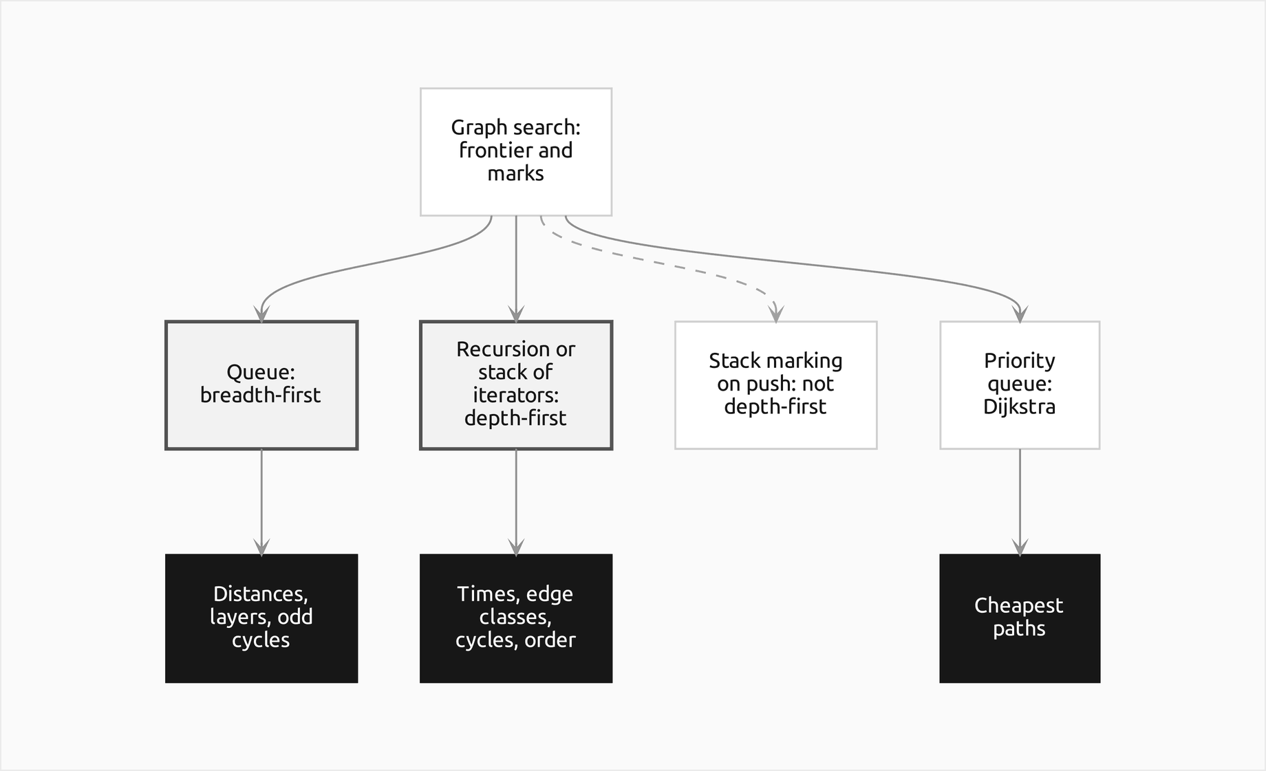
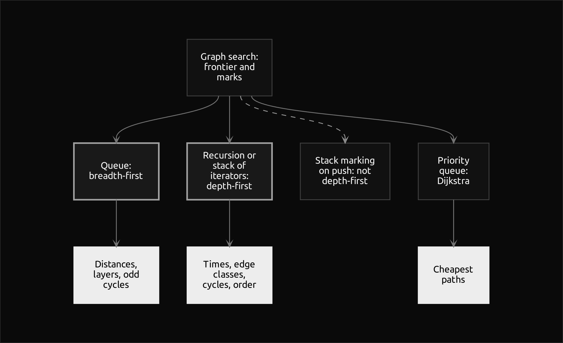
The diagram shows the one idea behind all of them. A search keeps a frontier of vertices it has discovered but not finished with, and the data structure holding that frontier decides the order of the visits and so the questions the search answers. The two outlined boxes are the subject of this page; the one reached by the dashed connector is a common imitation of the second, and the last one, ordered by distance, belongs to Single-source shortest paths.

How it works¶

Graphs as adjacency lists¶

A graph G = (V, E) has n vertices and m edges. In an undirected graph an edge {u, v} joins two vertices both ways; in a directed graph an edge (u, v) leads from its tail u to its head v. Searches spend their time asking one question, "what are the neighbours of this vertex?", and the representation that answers it best is the adjacency list: for every vertex, the list of its neighbours. An undirected edge appears in two lists, once at each end, so the lists hold 2m entries; a directed edge appears only in the list of its tail, m entries in all. Graphs and their representations compares this with adjacency matrices and edge lists; this page carries the small class it needs.

Graph in graph.py stores, for every vertex, a dictionary from neighbour to edge weight. A Python dictionary keeps the order in which keys were added, so it is an ordered adjacency list with constant-time edge lookups. The order matters more than it seems: neither search promises a particular visit order in general, only one that follows the order of the adjacency lists, so two correct programs given the same edges in a different order visit the vertices differently. Every result on this page, and every comparison with NetworkX, fixes the order by adding the edges in a stated order.

Searching with a frontier¶

Every vertex is in one of three states during a search. White means undiscovered. Gray means discovered but not finished: the vertex is on the frontier and some of its edges remain to be examined. Black means finished: all its edges have been examined. A search repeatedly takes a gray vertex, examines its edges, discovers the white vertices at their other ends, and turns the vertex black when nothing is left. Two rules keep it correct and linear. Each vertex must be marked the moment it is discovered, so that no other edge discovers it again, and each adjacency list must be read only once. The searches below differ only in which gray vertex they take next.

Breadth-first search¶

BFS takes the gray vertex that was discovered earliest, so its frontier is a first-in, first-out queue. It puts the source s in the queue with distance d[s] = 0, then repeats: dequeue a vertex u, and for each neighbour v that has not been discovered, set d[v] = d[u] + 1, record u as the parent π(v) of v, and enqueue v. It stops when the queue is empty. The code is short:

while queue:
    u = queue.popleft()
    for v in graph.adjacency[u]:
        if v in distance:
            continue
        distance[v] = distance[u] + 1
        parent[v] = u
        queue.append(v)

The distance map doubles as the mark. A vertex enters it, and the queue, the first time any edge reaches it, which is why no vertex is ever enqueued twice. collections.deque makes both ends O(1); a Python list used as a queue with pop(0) moves every remaining item one slot at each step, which the pitfalls measure.

Layers, the parent tree and fewest-edge paths¶

The distance δ(s, v) of a vertex is the smallest number of edges on any path from s to it:

The distance delta of s and v is the smallest number of edges on a path from s to v, and infinity when no path from s to v exists

Grouping the vertices by distance gives the layers. Layer 0 is the source alone, and layer k + 1 holds every vertex not in an earlier layer that has an edge from layer k:

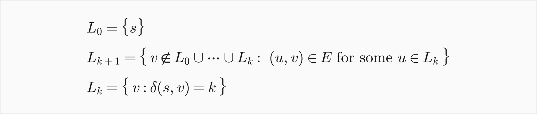
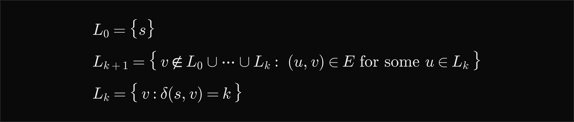
L 0 is the set containing s; L k plus 1 is the set of vertices v not in L 0 through L k with an edge u v for some u in L k; and L k is the set of vertices at distance k from s

BFS discovers the layers one after the other, and bfs_layers builds them exactly as the formula says, one list at a time without any queue; concatenated, they are the visit order of the queue version, which the tests check on hundreds of random graphs. The parent pointers form the BFS tree, a tree rooted at s that contains every reachable vertex, and walking parents back from any vertex t and reversing gives a path from s to t. Its length is d[t], and, as the next section proves, no path has fewer edges. Fewest-edge paths are rarely unique; BFS returns the one whose vertices it discovered first, so the neighbour order decides which. fewest_edge_path stops as soon as the target is discovered, because its distance is final at that moment.

Several sources can start at once. Putting all of them in the queue at distance 0 gives every vertex its distance to the nearest source, the multi-source BFS behind questions such as "how far is each cell from the nearest exit". And BFS restarted from every vertex not yet reached, in vertex order, visits the whole graph; in an undirected graph each restart opens a new connected component, the subject of Connected components.

Why the distances are right¶

The distance map is never too small: each value counts the edges of a real path, the one through the parents. The proof that it is never too large rests on two facts. The first is the triangle inequality for edge counts: one more edge reaches at most one step further.

The distance from s to v is at most the distance from s to u plus 1, for every edge u v with u reachable from s

The second is an invariant of the queue. At every moment the queue holds vertices in nondecreasing order of d, and the last is at most one more than the first:

For the queue v 1 to v r, d of v 1 is at most d of v 2 and so on up to d of v r, which is at most d of v 1 plus 1

It holds at the start, when the queue holds s alone. Dequeuing the head keeps it, and every vertex enqueued while u is processed gets d[u] + 1, which is at least everything in the queue and at most the new head's value plus one, because the new head is at least d[u]. So the values in the queue only grow, and over the whole run vertices are enqueued, and dequeued, in nondecreasing order of d. Now suppose some vertex ends with the wrong distance:

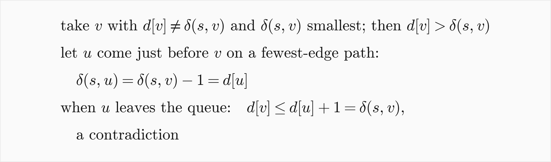
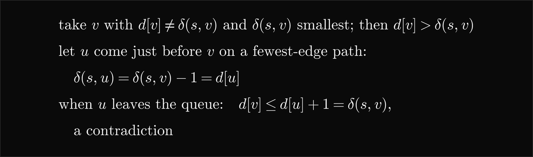
Take v with d of v different from delta of s and v, and with delta of s and v smallest; then d of v is greater than delta of s and v. Let u come just before v on a fewest-edge path: delta of s and u equals delta of s and v minus 1 equals d of u. When u leaves the queue, d of v is at most d of u plus 1, which equals delta of s and v, a contradiction Take v with d of v different from delta of s and v, and with delta of s and v smallest; then d of v is greater than delta of s and v. Let u come just before v on a fewest-edge path: delta of s and u equals delta of s and v minus 1 equals d of u. When u leaves the queue, d of v is at most d of u plus 1, which equals delta of s and v, a contradiction

The middle step uses minimality: u is closer to s than v, so its distance is right. The last step uses the queue: when u is dequeued, v is either undiscovered, and then receives d[u] + 1, or already discovered, and then it entered the queue before u left it, so its value is at most d[u] + 1. Either way d[v] ≤ δ(s, v), and with the opposite inequality, equality. The validity check bfs_violation turns the argument into code: every vertex one edge beyond its parent, and d[v] ≤ d[u] + 1 on every edge. A distance map with both properties cannot be beaten by any path.

Only when every edge counts the same¶

BFS counts edges. When edges carry weights, such as road lengths or prices, the path with the fewest edges and the cheapest path are different questions, and BFS answers only the first. On the road map of workloads.py, three simple routes lead from home to work. BFS returns home, park, work: two roads weighing 6 + 3 = 9. The route home, mill, port, work has three roads and weighs 2 + 4 + 2 = 8, and home, mill, farm, port, work has four roads and weighs 2 + 1 + 2 + 2 = 7, the cheapest: here every extra road makes the route cheaper. Reading a BFS path off a weighted graph and adding up its weights gives the weight of one particular path, not the minimum, and the result is right only by luck, when the graph happens to offer no cheaper detour. Cheapest paths with non-negative weights need Dijkstra's algorithm, whose frontier is a priority queue ordered by the distance found so far, and negative weights need Bellman-Ford; both are in Single-source shortest paths.

Two special cases keep the breadth-first idea. With small positive integer weights, replacing an edge of weight w by a chain of w unit edges makes BFS count weight, at the price of a larger graph:

The subdivided graph has n prime equal to n plus the sum over all edges of w of e minus 1 vertices, and m prime equal to the sum over all edges of w of e edges

On the road map the 7 roads become 19 vertices, and BFS finds 7 unit steps through home, mill, farm, port, work. With weights 0 and 1 only, 0-1 BFS replaces the queue by a deque: a vertex reached along a 0-edge has the same distance as its predecessor and goes to the front, one reached along a 1-edge goes to the back, and the deque stays sorted by distance as the BFS queue does. With tolls of 0 and 1 on the same roads, zero_one_bfs finds home, mill, farm, port, work with one toll, where the BFS route home, park, work pays two.

Testing bipartiteness¶

A graph is bipartite when its vertices can be split into two sides with every edge crossing between them, which is the same as colouring every vertex with one of two colours so that no edge joins two vertices of one colour. A cycle of odd length cannot be coloured that way, since the colours must alternate around it, and the converse holds as well:

G is bipartite if and only if G has a proper two-colouring, which holds if and only if G has no cycle of odd length

BFS proves the converse and tests the property in one pass. In an undirected graph an edge never skips a layer, because a neighbour of a vertex in layer k is discovered by the time that vertex is dequeued:

The distances of the two ends of an edge differ by at most 1, for every edge of an undirected graph

Colour each vertex by the parity of its distance. Then an edge between consecutive layers joins two colours, and the only edges that can join equal colours lie inside one layer. Such an edge {u, v}, together with the two tree paths from u and v up to their lowest common ancestor w, closes a cycle whose length is odd:

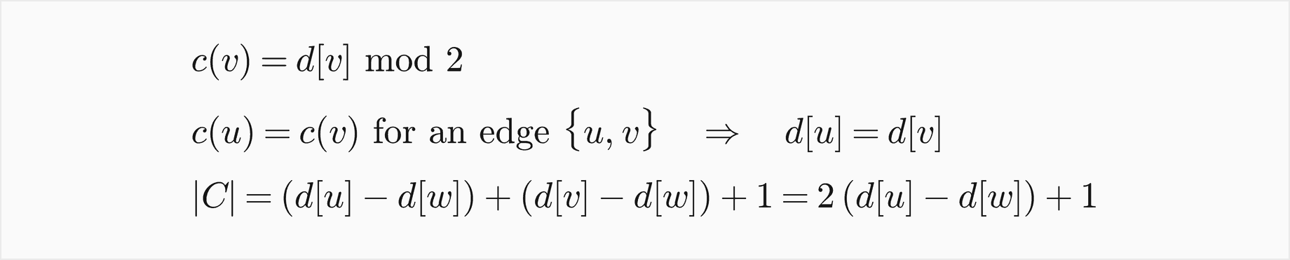
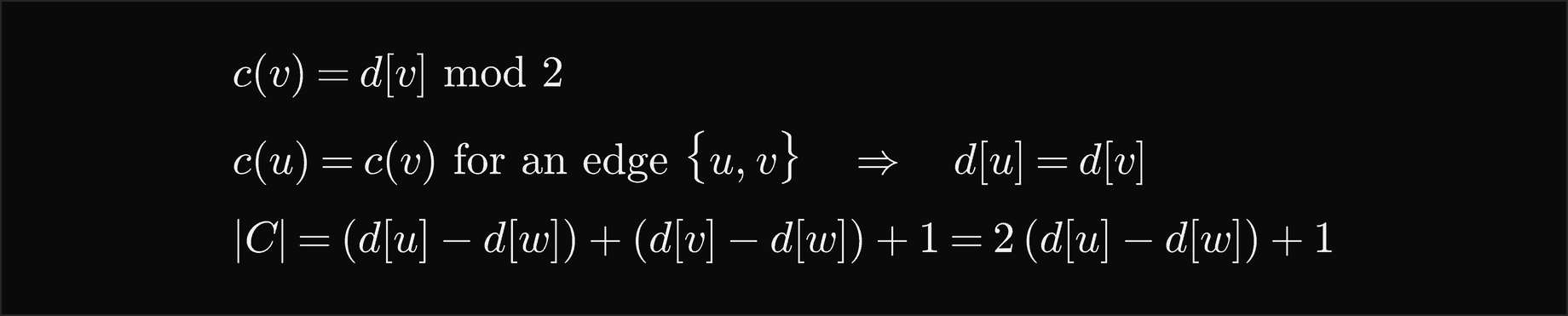
The colour of v is d of v mod 2; if an edge u v joins two vertices of the same colour then d of u equals d of v; and the cycle through the edge has length d of u minus d of w, plus d of v minus d of w, plus 1, which is 2 times d of u minus d of w, plus 1

So BFS either finishes with a proper colouring, which proves the graph bipartite, or finds an edge inside a layer and returns an odd cycle, which proves it is not. two_colouring returns the evidence in both cases. It must restart from every uncoloured vertex: an odd cycle in a component the first search never reached would otherwise go unnoticed. Two small facts are worth remembering: a single edge is bipartite, so the complete graphs on one and two vertices are bipartite while every larger complete graph is not, and a self-loop is an odd cycle of length one.

Depth-first search¶

DFS takes the gray vertex discovered most recently, and the natural way to write that is recursion. To visit u, mark it, then for each neighbour v in order: if v is white, visit v. Each call stays on the call stack until all its neighbours are done, so the stack of active calls is exactly the path from the root to the current vertex, the thread through the cave. Started from every white vertex in vertex order, the search covers the whole graph and its parent pointers form a depth-first forest, one tree per start.

def visit(u):
    clock += 1
    discovery[u] = clock
    for v in graph.adjacency[u]:
        if v not in discovery:
            parent[v] = u
            visit(v)
    clock += 1
    finish[u] = clock

The search is depth-first because of one rule, which every correct version obeys: the next vertex to be discovered is always an undiscovered neighbour of the most recently discovered vertex that still has one. dfs_order_violation in orders.py replays any visit order against that rule and says where it breaks.

Discovery and finish times¶

A single clock ticks once when a vertex is discovered and once when it is finished, so every vertex gets two times, d[v] and f[v], and together they use every number from 1 to 2n exactly once:

1 is at most d of v, which is less than f of v, which is at most 2n; and the set of all discovery and finish times is the set 1 to 2n

A call for v starts after the call of its parent and returns before it, so the time interval [d[v], f[v]] of a descendant lies inside that of its ancestor. Two unrelated vertices are processed one after the other, so their intervals do not meet. This is the parenthesis theorem: write an opening bracket at each discovery and a closing one at each finish, and the brackets nest properly.

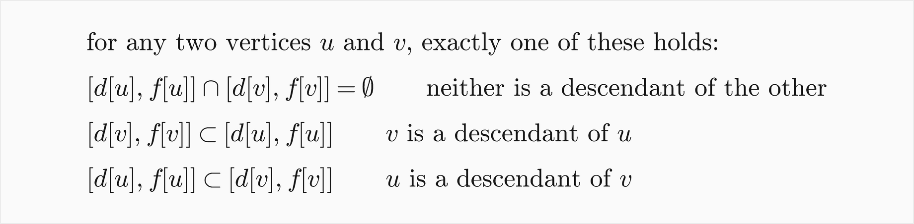
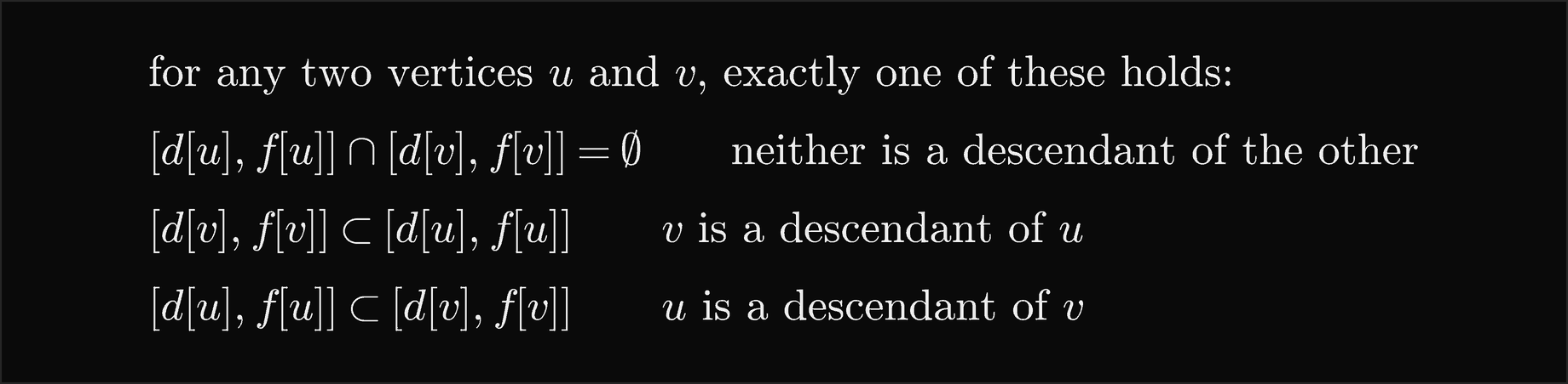
For any two vertices u and v, exactly one of these holds: the intervals of u and v are disjoint and neither is a descendant of the other; the interval of v lies inside that of u and v is a descendant of u; or the interval of u lies inside that of v and u is a descendant of v

Read as a test, it turns ancestry into two comparisons, which DFSResult.is_ancestor uses:

v is a proper descendant of u if and only if d of u is less than d of v, which is less than f of v, which is less than f of u

The times of the worked example below, written as brackets, read (a (b (c c) (e e) b) (d (f f) d) a) (g (h h) g). The finish order, the postorder, is the other output that matters: in a directed graph without cycles, every edge goes from a vertex that finishes later to one that finishes earlier, so the reversed postorder is a topological order, the method of Topological sorting.

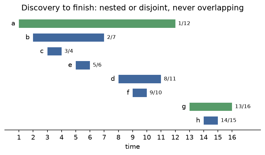
Eight horizontal bars, one per vertex in discovery order, from its discovery to its finish time: a from 1 to 12 and g from 13 to 16 in green as roots; inside a, b from 2 to 7 with c from 3 to 4 and e from 5 to 6, then d from 8 to 11 with f from 9 to 10; inside g, h from 14 to 15

Every bar lies inside the bar of each of its ancestors and apart from every bar it is not related to; no two bars overlap partially. That is the parenthesis theorem drawn for the eight vertices of the worked example.

The white-path theorem¶

Which vertices end up below u in the forest? Exactly those that could be reached from u through undiscovered vertices at the moment u was discovered:

v is a descendant of u in the depth-first forest if and only if, at time d of u, some path leads from u to v through white vertices only

If v is a descendant, the tree path from u to v consists of vertices discovered after u, so they were white at time d[u]. Conversely, suppose a white path from u to v exists but v is not a descendant, and take the first vertex x on the path that is not one; its predecessor on the path is u or a descendant of u, and that vertex examines the edge to x before it finishes, so x is discovered before u finishes, inside u's interval, and is a descendant after all. The theorem explains what DFS from a vertex finds, and it is the key step in the correctness of strongly connected components and topological sorting. white_path_violation checks it directly, by searching from every vertex through later-discovered vertices only; it found no counterexample in 200 random graphs.

Classifying edges¶

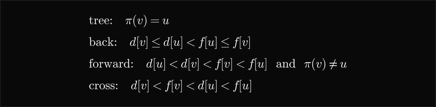
In a directed graph DFS sorts every edge (u, v) into one of four classes, by the state of v at the moment u examines the edge:

If v is white the edge is a tree edge, if v is gray it is a back edge; if v is black and d of u is less than d of v it is a forward edge, and if v is black and d of v is less than d of u it is a cross edge

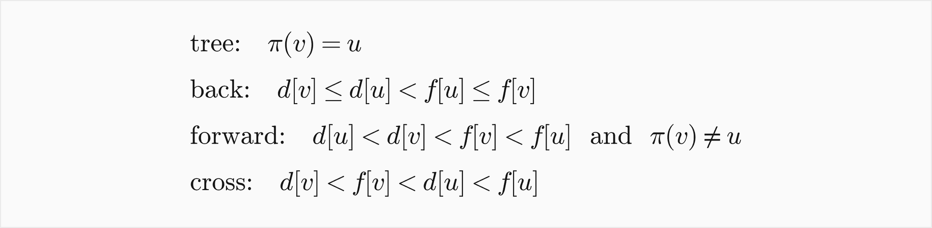
A white v becomes u's child: a tree edge. A gray v is still on the current path, an ancestor of u: the edge points back up the tree, a back edge, and a self-loop counts as one. A black v discovered after u must be a descendant of u that is already finished, reached through another child: a forward edge. A black v discovered before u lies in a subtree that was finished before u was even discovered: a cross edge, which always points from later to earlier in discovery order. After the search the same classes can be read off the times alone, which is how classify_by_times checks classify_on_arrival:

Tree: the parent of v is u. Back: d of v is at most d of u, which is less than f of u, which is at most f of v. Forward: d of u is less than d of v, which is less than f of v, which is less than f of u, and the parent of v is not u. Cross: d of v is less than f of v, which is less than d of u, which is less than f of u Tree: the parent of v is u. Back: d of v is at most d of u, which is less than f of u, which is at most f of v. Forward: d of u is less than d of v, which is less than f of v, which is less than f of u, and the parent of v is not u. Cross: d of v is less than f of v, which is less than d of u, which is less than f of u

An undirected edge appears in two adjacency lists, so the search meets it twice. Seen from a child, the edge to the parent is the tree edge already taken, and the code skips it; seen from an ancestor, an edge to a finished descendant was already classified from the other end, as a back edge. Forward and cross edges cannot occur. When the search at u meets a neighbour v that is already finished, v must be a descendant of u: had v been discovered before u, then u, white and adjacent to v, would have been discovered inside v's call, and v could not finish while u is still being searched. Every undirected edge is therefore a tree edge or a back edge, which fixes the counts:

In an undirected graph every edge is a tree edge or a back edge; there are n minus c tree edges and m minus n plus c back edges, with c trees in the forest

On a random undirected graph with 200 vertices and 300 edges the search made 10 trees, 190 tree edges and 110 back edges, as the formula predicts. On a random directed graph with 200 vertices and 800 edges it made 8 trees with 192 tree edges, 268 back, 177 forward and 163 cross edges.

Detecting cycles¶

A back edge (u, v) closes a cycle: the tree path from v down to u, then the edge back to v. Conversely, if the graph has a cycle, let v be the first vertex of the cycle to be discovered; at that moment the rest of the cycle is white and reachable along it, so by the white-path theorem the vertex u just before v on the cycle becomes a descendant of v, and the edge (u, v) is examined while v is still gray: a back edge.

G has a cycle if and only if a depth-first search of G finds a back edge

find_cycle is that theorem in code: it runs the search and turns the first back edge into the list of vertices of the cycle. For an undirected graph the same holds, with the edge to the parent excluded, which the classification already does. The two classic errors are both about the wrong notion of "seen". A directed check that reports a cycle on any edge to a visited vertex mistakes forward and cross edges for cycles, and calls a simple diamond a, b, d and a, c, d cyclic. An undirected check that does not skip the parent finds the tree edge it just used and calls every tree cyclic.

Depth-first search without recursion¶

Python allows about a thousand nested calls, so the recursive search fails on any graph with a path of that many vertices, which a grid or a road network has easily. The cure is to keep the call stack ourselves. A recursive call holds two things: the vertex and how far it has got through its adjacency list. An iterator over the list holds the second, so the explicit stack holds (vertex, iterator) pairs:

stack = [(root, iter(graph.adjacency[root]))]
while stack:
    u, neighbours = stack[-1]
    for v in neighbours:
        if v not in discovery:
            discover(v)
            stack.append((v, iter(graph.adjacency[v])))
            break
    else:
        stack.pop()
        finish(u)

The for loop resumes u's list where it stopped. Finding a white neighbour, pushing it and breaking out is the recursive call; running out of neighbours, popping and finishing u is the return. iterative_dfs produces the same times, forest, edge classes and even the same trace as dfs, which the tests compare on 200 random graphs, and it handles a path of 50000 vertices that the recursive version cannot.

There is a second correct way, with a stack of plain vertices. Push the root; pop a vertex, skip it if it is already visited, otherwise visit it and push its unvisited neighbours in reverse order, so that the first one listed comes off first. The newest entries always lie on top, so the search continues from the most recently visited vertex that still has an unvisited neighbour, exactly the depth-first rule, and stack_preorder produces the same preorder and the same tree as the recursive search. It gives no finish times without more bookkeeping, and a vertex can sit in the stack once for every edge that reached it while it was unvisited, so the stack can grow to about m entries: 2726 entries on a directed graph with 300 vertices and 6000 edges, against a deepest path of 279 for the iterator stack.

Pushes are at most n when marking on push; when marking on pop, pushes are at most 1 plus m for a directed graph and at most 1 plus 2m for an undirected one

The stack search that marks vertices when it pushes them, the subject of the next section, keeps its stack within n entries, and pays for that by giving up the depth-first order.

The stack search that is not depth-first¶

A third version is shown very often under the name DFS: replace BFS's queue by a stack and keep everything else, so each vertex is marked when it is pushed. Pop a vertex, visit it, and push every unmarked neighbour, marking them all at once. It visits every reachable vertex exactly once, its stack never holds more than n vertices, and it is a perfectly good way to answer "what can I reach?". It is not a depth-first search. A neighbour marked early is never pushed again from a deeper vertex, so when the search reaches a vertex whose remaining neighbours are all marked but still waiting lower in the stack, it moves on to whatever lies on top, which need not be adjacent to the vertex it just left.

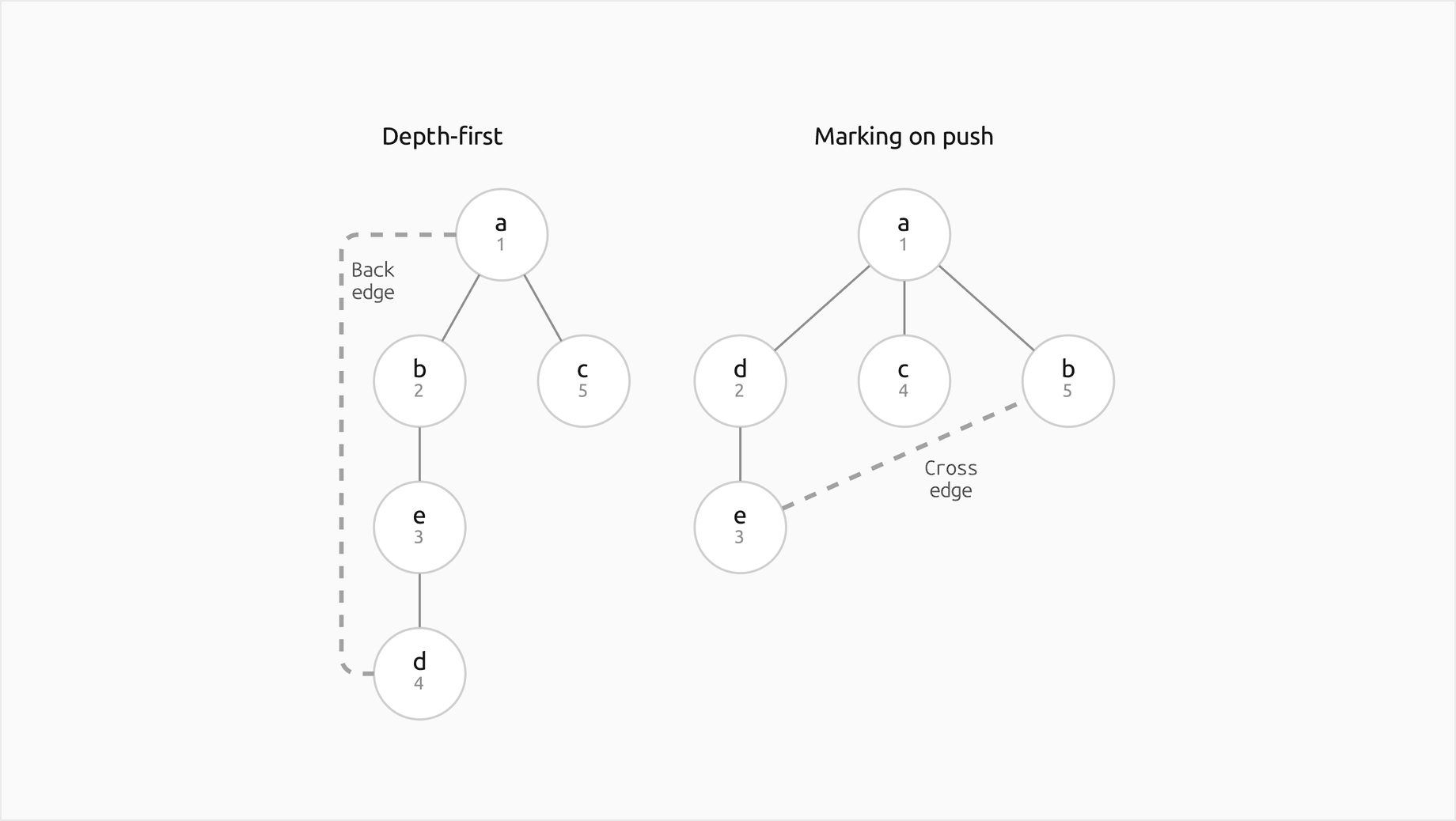
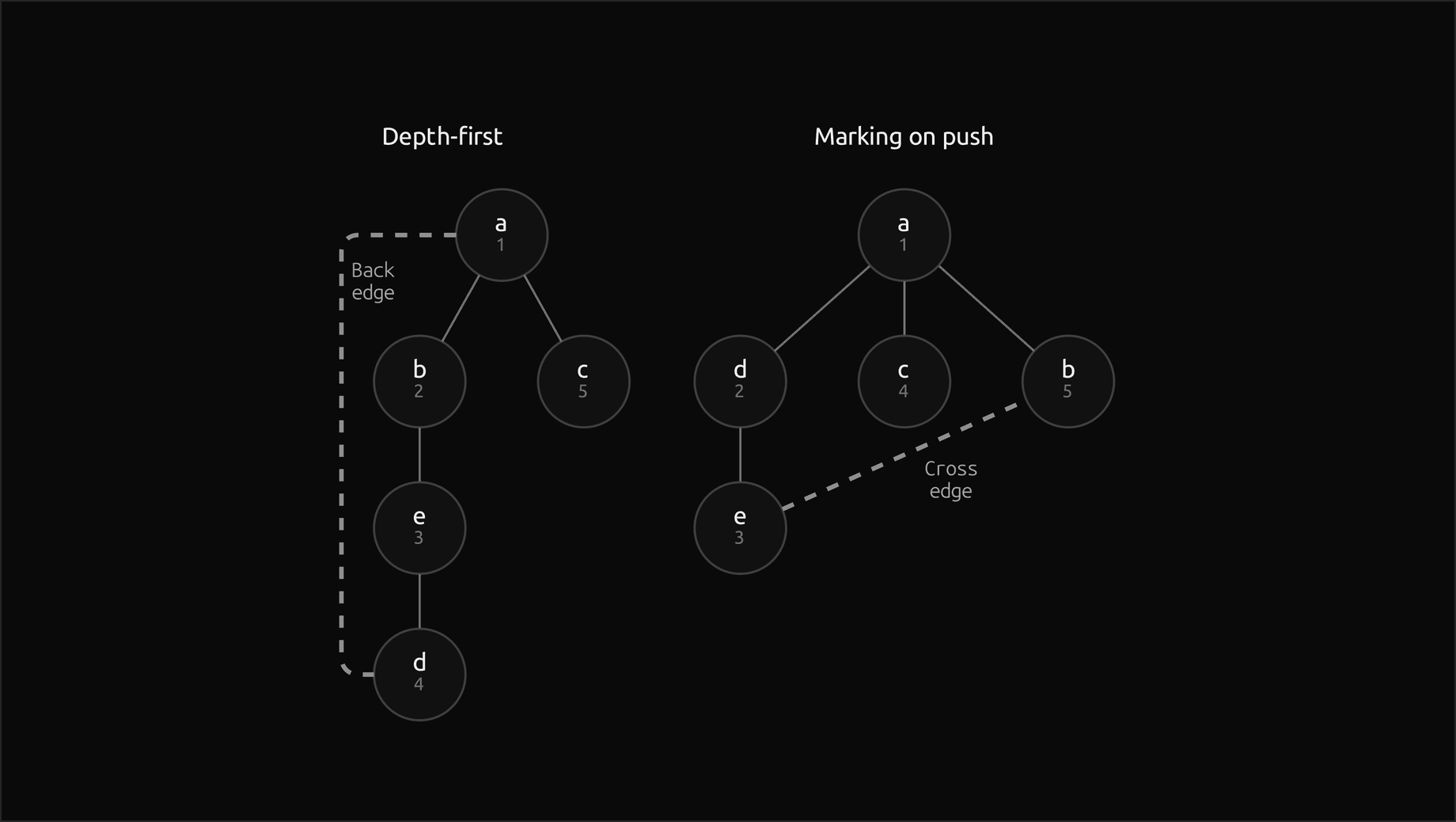
The graph is a four-cycle a, b, e, d with a pendant vertex c, and a lists its neighbours as b, c, d. Marking on push, a pushes and marks b, c and d; d comes off, and pushes e; e comes off, but its other neighbour b is already marked, so nothing is pushed; then c comes off, although c is not adjacent to e and e still has the unvisited neighbour b. The order a, d, e, c, b is not the order of any depth-first search, whatever the neighbour order, and pushing the neighbours in reverse gives a, b, e, c, d, which fails in the same way. The tree it leaves is no depth-first tree either: the edge e to b joins two vertices neither of which is an ancestor of the other, a cross edge, which an undirected depth-first search can never produce. Anything built on DFS's structure, times, edge classes, cycle detection, topological order, strongly connected components, articulation points, breaks when given this search. On 887 random graphs with at least five vertices its order failed the depth-first rule on 677, a share of 0.7632.

Implicit graphs¶

Many graphs are never stored. The cells of a maze, the positions of a puzzle and the words of a word game are vertices whose neighbours a function computes on demand. The searches need only that function, so bfs_implicit and dfs_implicit take a start state, a neighbour function and an optional goal test, and they keep only the states they have actually reached, in a dictionary of distances and parents. States must be hashable: tuples for grid cells and puzzle positions, strings for words.

A grid becomes a graph with four moves per cell, up, right, down and left, within the bounds and not into a wall. On the small maze in workloads.py, BFS finds the 12 steps down the left side and along the bottom, while DFS, which tries right before down, wanders across the top, back through the middle, along the bottom and up and down the right-hand columns for 26 steps. A puzzle becomes a graph of positions. In the water-jug puzzle, with jugs of 4 and 9 litres, a tap and a drain, each move fills a jug, empties one, or pours one into the other until the first is empty or the second full, and the question is how to measure exactly 6 litres. BFS finds the shortest solution, 8 moves: fill the 9, pour into the 4 to leave 5, empty the 4, pour again to leave 1, empty the 4, pour the 1 across, fill the 9, and top up the 4 from it, which leaves 6. It reached 18 of the 26 positions that can occur at all, out of a bound of 50:

The number of states is at most A plus 1 times B plus 1: states x, y with x from 0 to A and y from 0 to B

The sample project adds word ladders, where two words are neighbours when they differ in one letter, and computes those neighbours through a dictionary of patterns rather than by comparing every pair:

Patterns stored: L times the number of words, for words of length L; neighbours of one word: L lookups instead of the number of words minus 1 comparisons

Two words that share a pattern differ only in its blank position, and two different words share at most one pattern, so the buckets list every neighbour of a word exactly once.

Cost¶

Every vertex and every edge once¶

Both searches enqueue or discover each vertex once and read each adjacency list once, when the vertex is dequeued or visited. The work is one step per vertex plus one per adjacency entry, and the handshake identity counts the entries:

The sum of the degrees of all vertices is 2m in an undirected graph; the sum of the out-degrees is m in a directed graph

So a full traversal costs

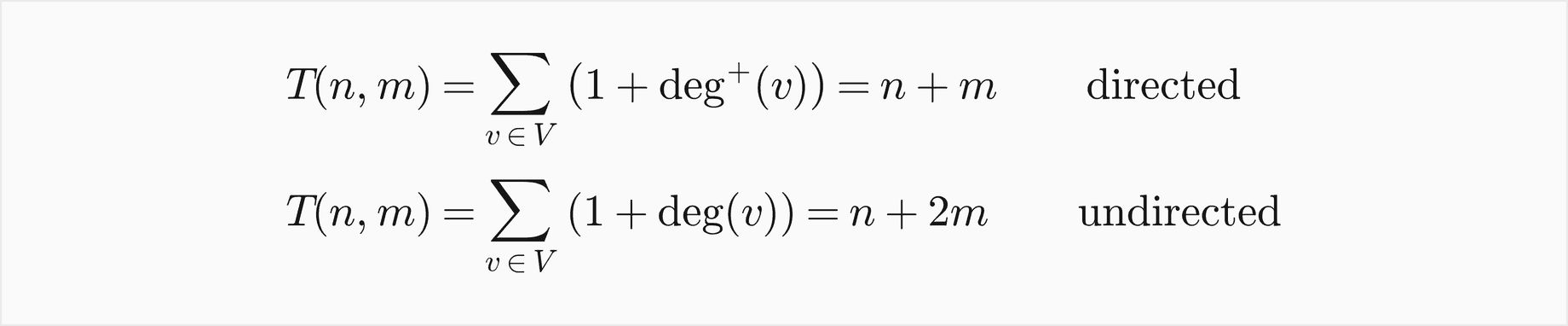
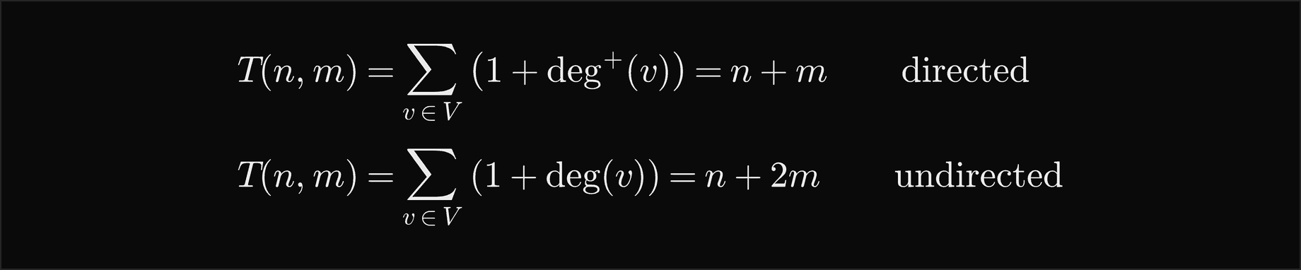
T of n and m is the sum over all vertices of 1 plus the out-degree, which is n plus m, for a directed graph; and the sum of 1 plus the degree, which is n plus 2m, for an undirected graph

which is Θ(n + m), linear in the size of the input, and nothing faster is possible when the whole graph must be read. The bound is worst case, not amortized or expected, for both searches and all their variants above. It assumes O(1) marks: a dictionary or a list of flags. A mark kept in a list searched by in costs Θ(n) per test and turns the search quadratic. A search from one source costs only the size of the part it reaches, and one that stops at a target, as fewest_edge_path does, can cost much less.

Memory is Θ(n) for the marks, distances, parents and times, plus the frontier, which the next sections measure. The representation itself takes Θ(n + m) with adjacency lists.

Adjacency matrices¶

With an adjacency matrix, finding the neighbours of a vertex means reading its whole row, n cells, however few neighbours it has:

T of n is the sum over all vertices of n, which is n squared

That is Θ(n²) for every graph, sparse or dense. The bounds in older texts written as O(n²) for BFS and DFS assume this representation, or a graph so dense that m is close to n²; with adjacency lists, the bound is n + m.

Counted work¶

The example traversal_costs.py traverses random directed graphs completely and counts vertices visited plus adjacency entries read, and, for the matrix version, cells read.

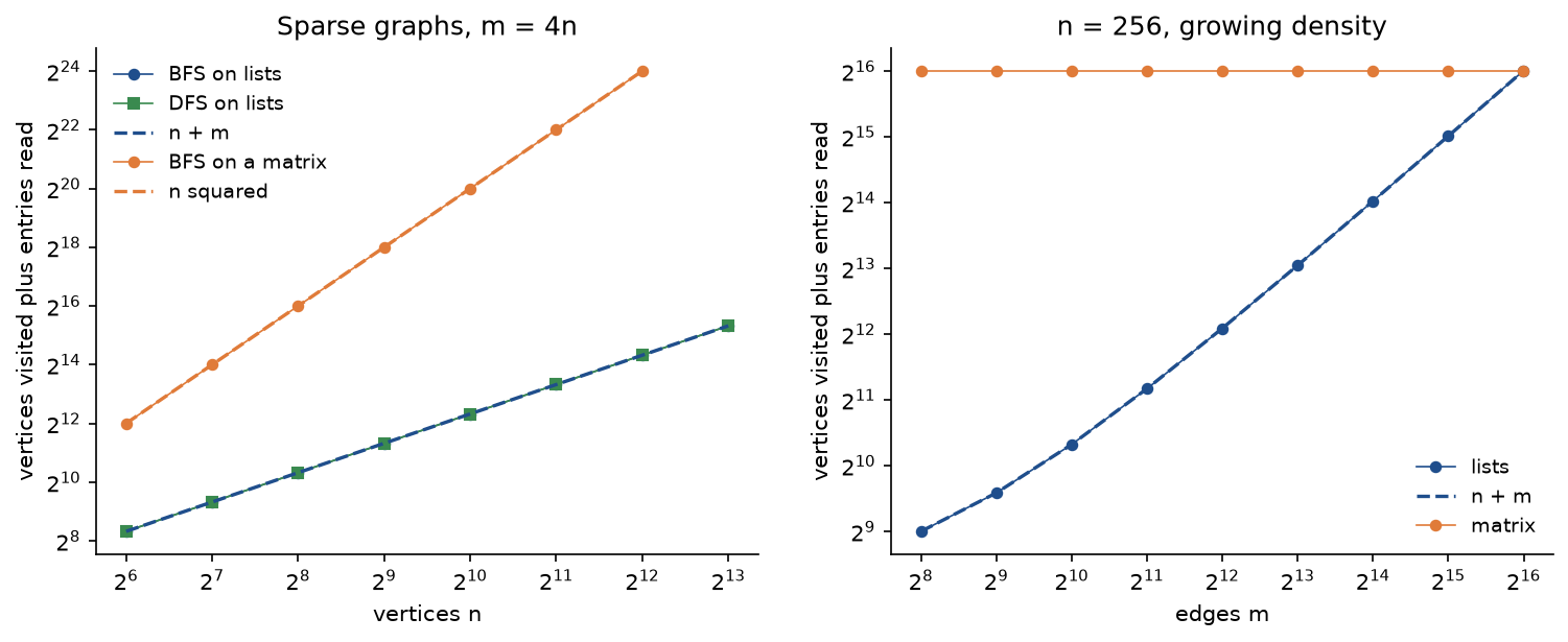
The counts equal the predictions exactly, not approximately: at n = 8192 both searches did 40960 units of work, 8192 vertices plus 32768 edges. The matrix version read 16777216 cells at n = 4096, where the lists needed 20480 steps, about 819 times fewer. The right panel shows that the lists never lose on this count: they meet the matrix only when the graph is complete, m = n(n − 1). A matrix earns its place elsewhere, in O(1) edge tests and in dense numerical work, as in All-pairs shortest paths.

How large the frontier grows¶

Both searches use Θ(n) memory in the worst case, but on a given graph their frontiers can differ enormously, and which one is smaller depends on the shape of the graph. BFS holds about one layer at a time, so its queue is as wide as the widest layer; DFS holds one path, so its stack is as deep as the longest path it follows.

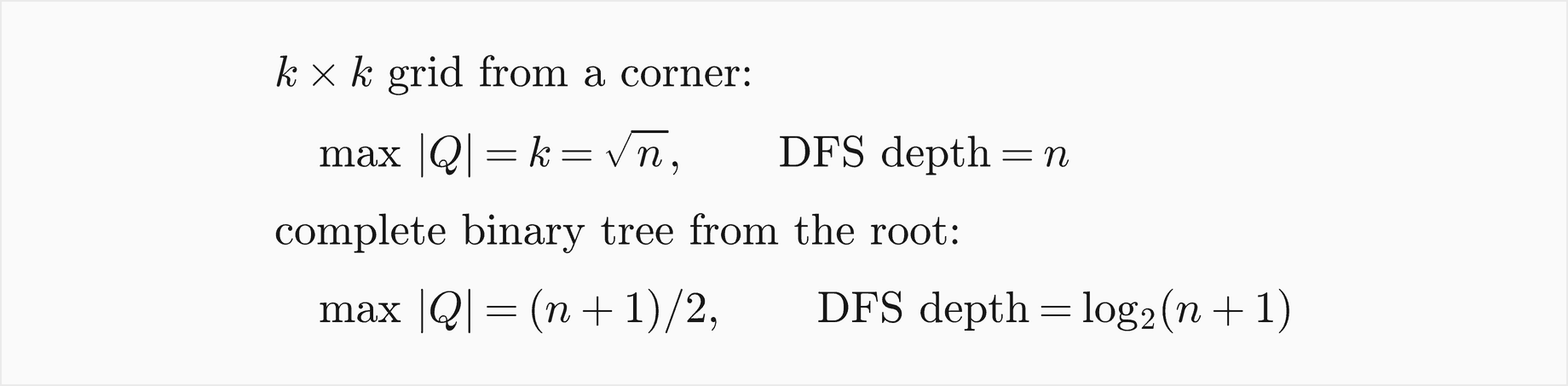
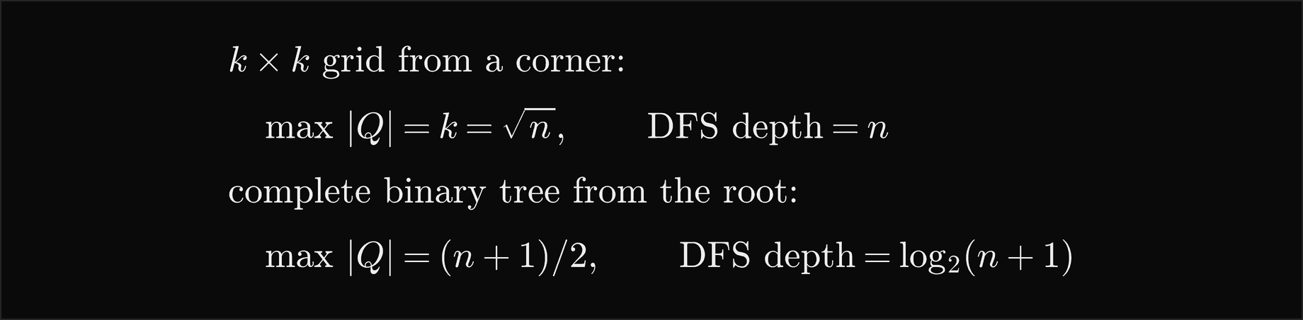
For a k by k grid searched from a corner, the largest queue is k, the square root of n, and the DFS depth is n; for a complete binary tree searched from the root, the largest queue is n plus 1 over 2 and the DFS depth is log base 2 of n plus 1

The example measures both on square grids from a corner and on complete binary trees from the root.

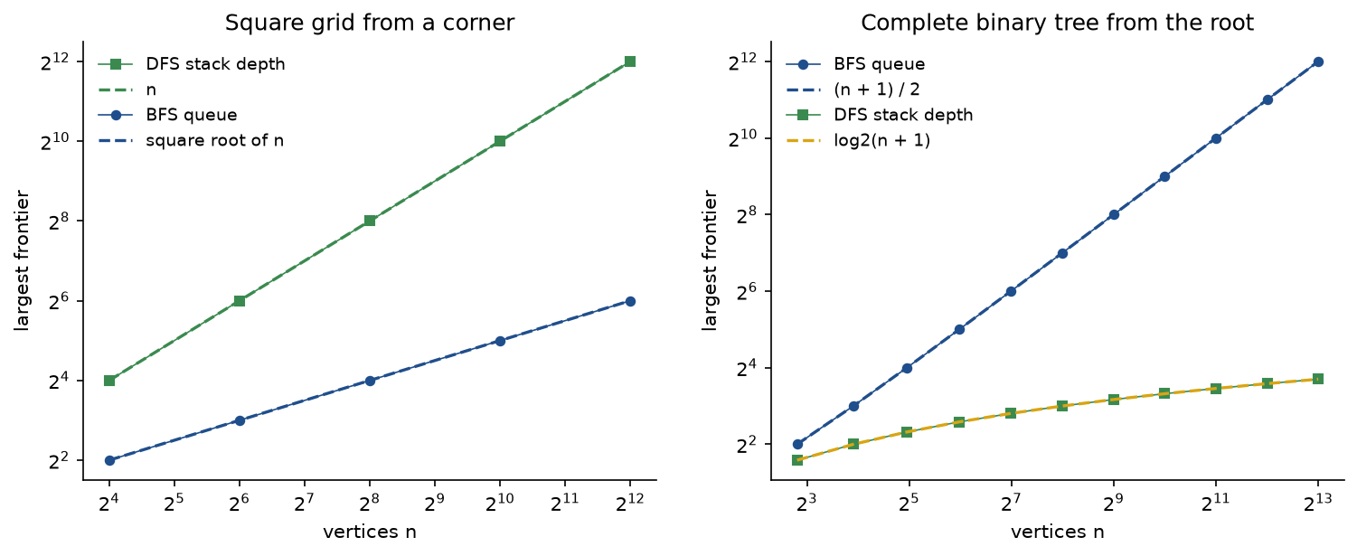
Two log-log panels of the largest frontier against n. Left, square grids from a corner for n from 16 to 4096: the DFS stack depth equals n, on its dashed line, while the BFS queue equals the square root of n, from 4 to 64. Right, complete binary trees for n from 7 to 8191: the BFS queue equals n plus 1 over 2, from 4 to 4096, while the DFS stack depth equals log2 of n plus 1, from 3 to 13

On a grid the BFS queue never exceeds the side length, 64 for 4096 cells, while DFS snakes through every cell in one path and holds all 4096 on its stack. On a binary tree it is the other way round: BFS holds the 4096 leaves at once, while DFS never holds more than the 13 vertices of one root-to-leaf path. Neither search is the memory-friendly one in general.

Recursion depth in Python¶

The recursive DFS needs one Python frame per vertex on the current path, so its depth equals the height of the depth-first tree plus one, which can reach n. CPython stops at sys.getrecursionlimit(), 1000 by default, counting the frames already in use. A path of 900 vertices works; one of 1000 raises RecursionError, as does every larger grid, long chain or large maze. Raising the limit with sys.setrecursionlimit only moves the wall, and too high a limit can crash the interpreter when the C stack runs out. The library code here never changes the limit. The recursive dfs is kept because it is the clearest statement of the algorithm and its traces are the ones to learn; iterative_dfs, which gives identical results, is the one to use on real data, and find_cycle uses it for that reason.

Worked example¶

Every step below is printed by examples/worked_example.py and asserted by tests/test_worked_example.py.

The graph¶

The undirected graph has ten vertices, trees in a park joined by footpaths, and thirteen edges, added in this order: oak ash, oak elm, ash fir, ash yew, elm fir, elm box, fir bay, yew box, yew bay, box fig, bay gum, fig gum, fig ivy. That order fixes the adjacency lists:

oak: ash, elm
ash: oak, fir, yew
elm: oak, fir, box
fir: ash, elm, bay
yew: ash, box, bay
box: elm, yew, fig
bay: fir, yew, gum
fig: box, gum, ivy
gum: bay, fig
ivy: fig

BFS from oak, step by step¶

The queue is written front first, as it stands after each step.

Start: oak gets distance 0. Queue [oak].
Dequeue oak. Its neighbours ash and elm are new: each gets distance 1 and parent oak. Queue [ash, elm].
Dequeue ash. oak was reached before; fir and yew are new, distance 2, parent ash. Queue [elm, fir, yew].
Dequeue elm. oak and fir were reached before; box is new, distance 2, parent elm. Queue [fir, yew, box].
Dequeue fir. ash and elm were reached before; bay is new, distance 3, parent fir. Queue [yew, box, bay].
Dequeue yew. All three neighbours ash, box and bay were reached before. Queue [box, bay].
Dequeue box. elm and yew were reached before; fig is new, distance 3, parent box. Queue [bay, fig].
Dequeue bay. fir and yew were reached before; gum is new, distance 4, parent bay. Queue [fig, gum].
Dequeue fig. box and gum were reached before; ivy is new, distance 4, parent fig. Queue [gum, ivy].
Dequeue gum, then ivy: every neighbour was reached before, and the queue empties.

The search visited 10 vertices and read 26 adjacency entries, 2m for 13 edges. The queue never held more than 3 vertices. Note the step at elm: fir is already in the queue, discovered from ash, so the edge elm fir does not change fir's parent or distance; the same happens to bay at yew. Changing the parent there is a common hand-tracing slip; the first discovery is final.

Layers, paths and an odd cycle¶

The layers are {oak}, {ash, elm}, {fir, yew, box}, {bay, fig} and {gum, ivy}, and the parents are ash and elm from oak, fir and yew from ash, box from elm, bay from fir, fig from box, gum from bay and ivy from fig. Walking back from gum gives the fewest-edge path oak, ash, fir, bay, gum of 4 edges. It is one of four: oak, elm, fir, bay, gum, then oak, ash, yew, bay, gum, and oak, elm, box, fig, gum are just as short, and BFS returns the first because it goes through the vertices discovered first: ash before elm, fir before yew and bay before fig.

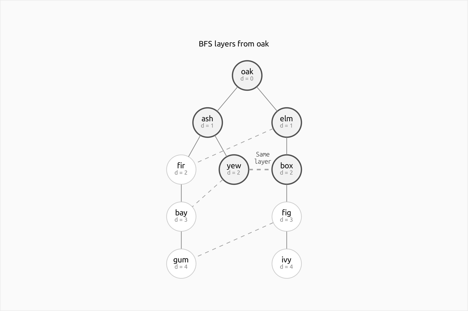
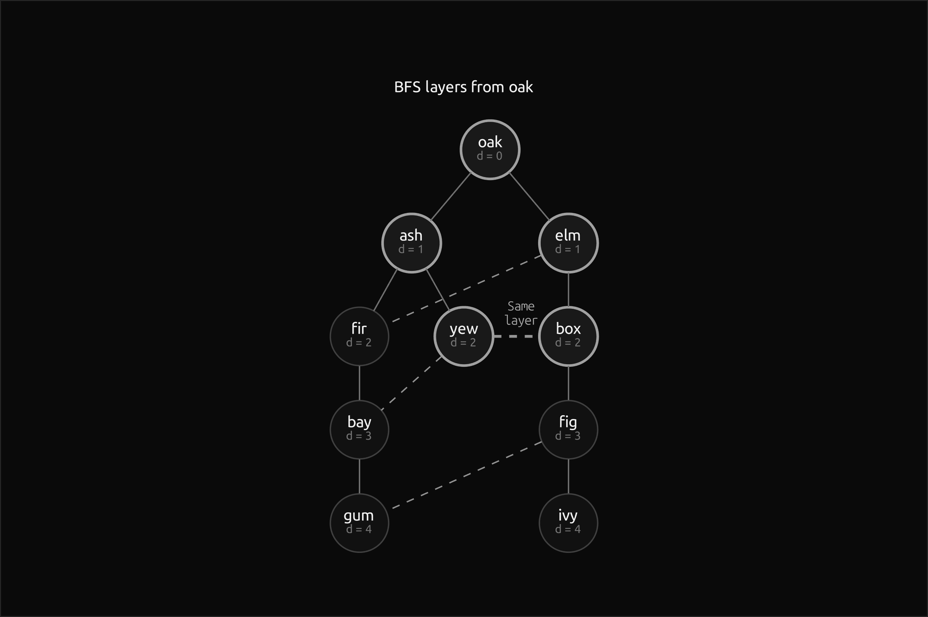
Three of the four non-tree edges join consecutive layers, as every edge of an undirected graph must, and one, yew box, lies inside layer 2. Colouring by parity puts yew and box both on colour 0, so the graph is not bipartite. two_colouring finds the conflict when it dequeues yew and returns the edge yew box and the cycle oak, ash, yew, box, elm: the tree paths from yew and box meet at oak, two edges each, plus the edge yew box, a cycle of length 2 · (2 − 0) + 1 = 5.

DFS from oak on the same graph visits oak, ash, fir, elm, box, yew, bay, gum, fig, ivy. Its tree is a single path through all ten vertices, of height 9 against 4 for the BFS tree, and its four non-tree edges, elm oak, yew ash, bay fir and fig box, all lead from a vertex to one of its ancestors.

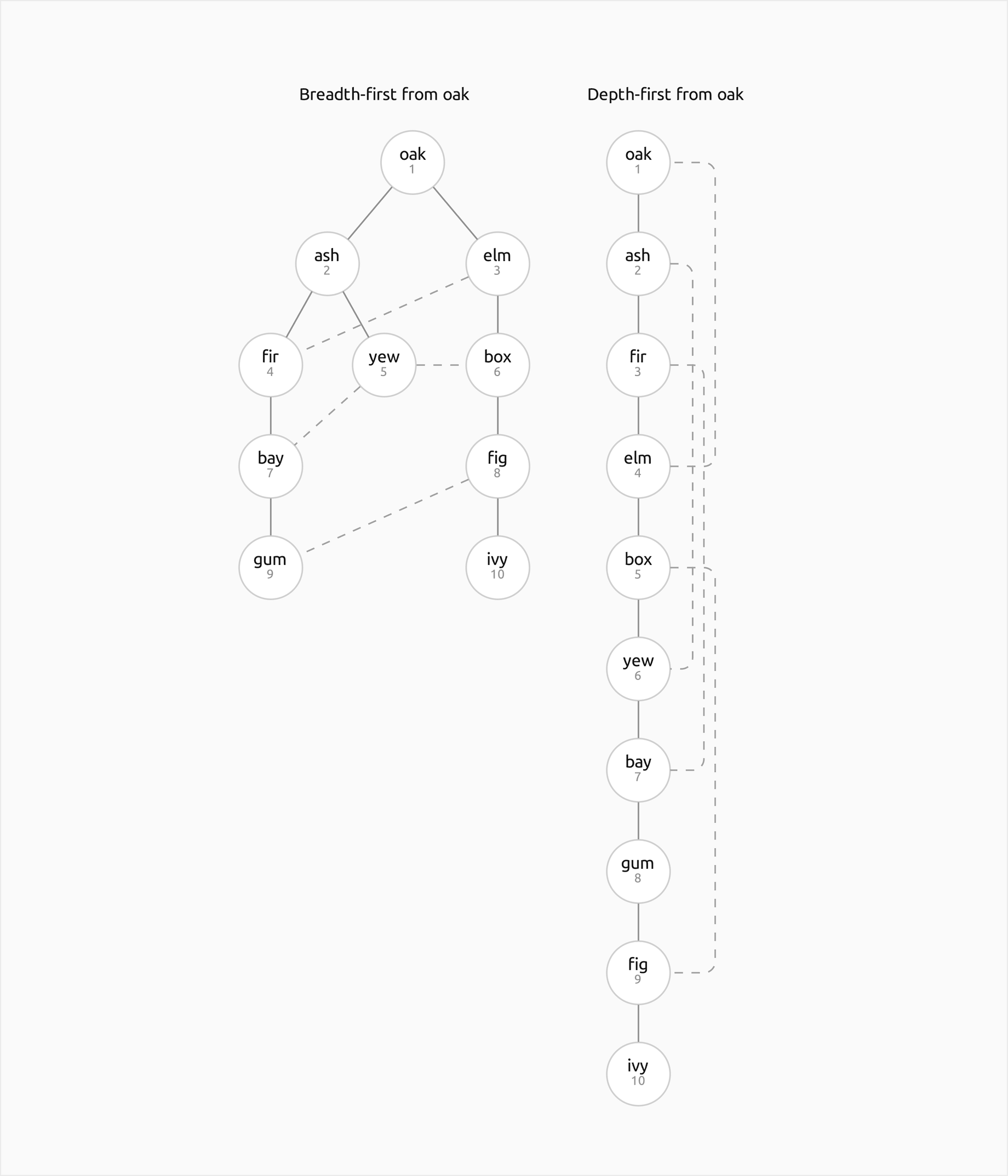
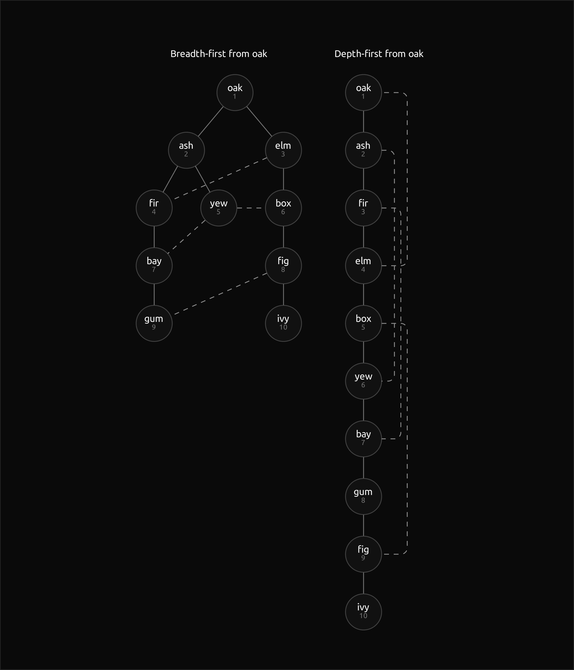
The same graph, two shapes. BFS keeps every tree path as short as possible, so its tree is wide and shallow. DFS goes as deep as it can before turning back, so here its tree is a single path, and every dashed edge in it joins a vertex to an ancestor.

DFS of a directed graph¶

The directed graph has eight vertices and twelve edges:

a: b, c, d
b: c, e
c: a
d: e, f
e: c
f: no edges out
g: h, d
h: g

DFS runs in vertex order. Each line gives the clock value and what happens:

1: discover a. Edge a to b: b is white, a tree edge.
2: discover b. Edge b to c: tree edge.
3: discover c. Edge c to a: a is gray, a back edge, and a cycle a, b, c.
4: finish c. Back in b, edge b to e: tree edge.
5: discover e. Edge e to c: c is black and was discovered before e, a cross edge.
6: finish e. 7: finish b. Back in a, edge a to c: c is black and was discovered after a, a forward edge.
Edge a to d: tree edge. 8: discover d. Edge d to e: e is black and earlier, a cross edge. Edge d to f: tree edge.
9: discover f; it has no edges. 10: finish f. 11: finish d. 12: finish a.
g is still white, so a new tree starts. 13: discover g. Edge g to h: tree edge. 14: discover h. Edge h to g: g is gray, a back edge.
15: finish h. Edge g to d: d is black and earlier, a cross edge. 16: finish g.

The intervals are a 1 to 12, b 2 to 7, c 3 to 4, e 5 to 6, d 8 to 11, f 9 to 10, g 13 to 16 and h 14 to 15, the postorder is c, e, b, f, d, a, h, g, and the search visited 8 vertices and read 12 adjacency entries. The classes are 6 tree edges (8 vertices minus 2 trees), 2 back edges, 1 forward edge and 3 cross edges. The two back edges reveal the two cycles, and find_cycle reports the first, a, b, c.

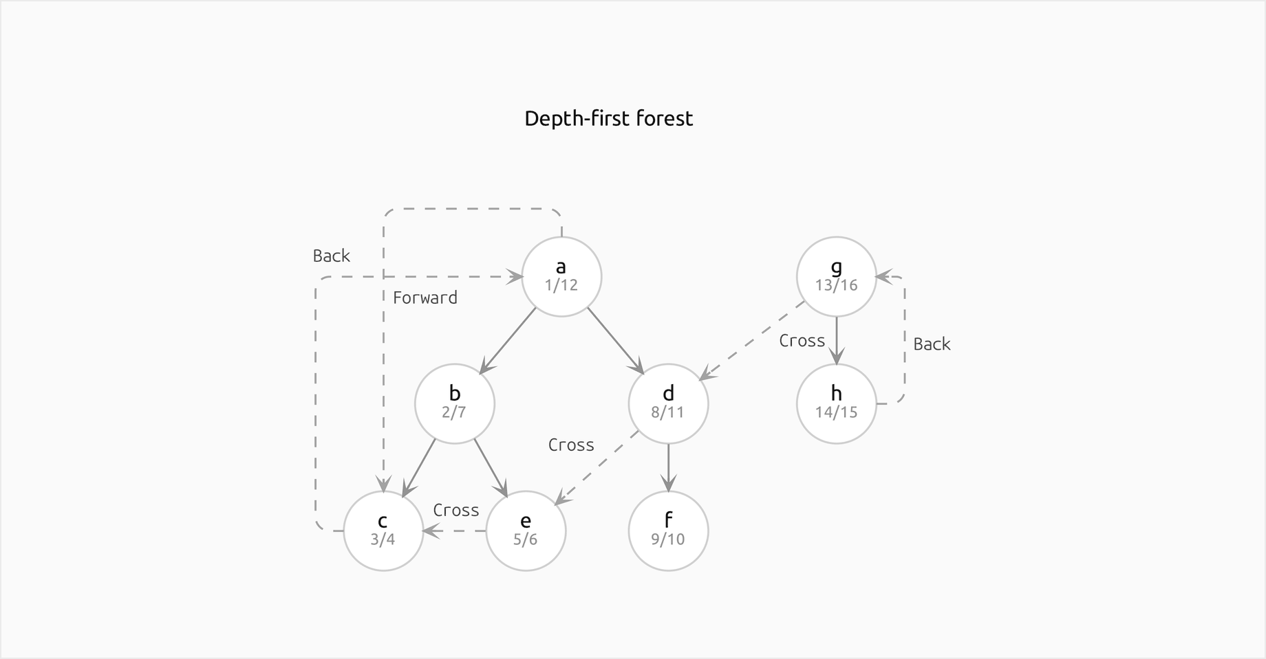
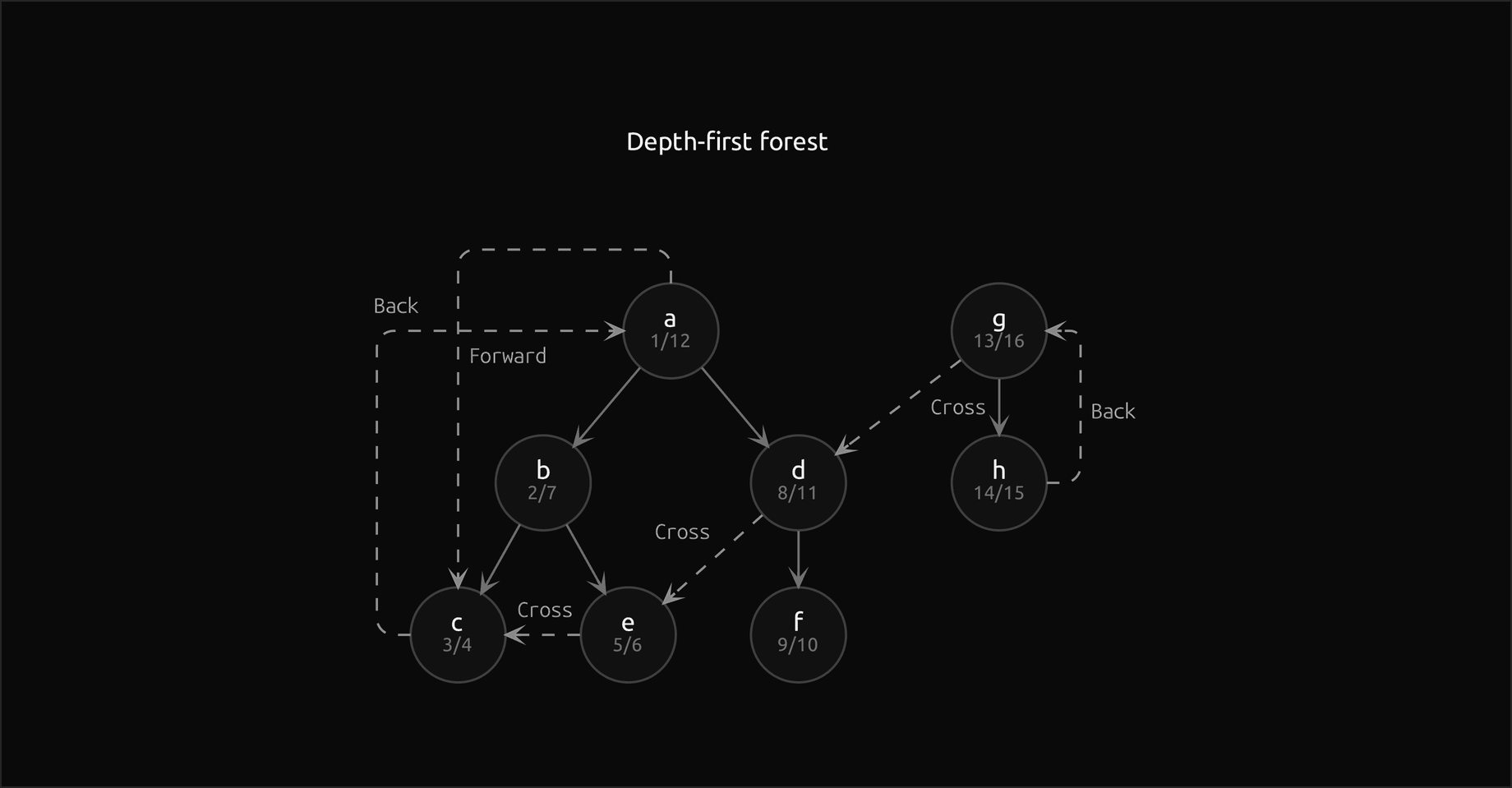
Read the classes off the picture with the times: the back edges point to a vertex whose interval contains the tail's, the forward edge to a vertex whose interval lies inside the tail's, and every cross edge points to the left, to a vertex that finished before its tail was discovered. The most common hand-tracing errors on such a graph are calling a to c a cross edge because c is black, which ignores that c was discovered after a, and forgetting the second tree at g.

The stack search on the same graph¶

The search that marks vertices when it pushes them runs differently on the same graph. The stack is written bottom first.

Push a. Pop a and visit it; push b, c and d, marking all three. Stack [b, c, d].
Pop d and visit it; push e and f. Stack [b, c, e, f].
Pop f and visit it. Stack [b, c, e].
Pop e and visit it; c is already marked. Stack [b, c].
Pop c and visit it; a is marked. Pop b and visit it; c and e are marked.
Push g, pop it and visit it; push h; pop h and visit it.

Its order is a, d, f, e, c, b, g, h, against a, b, c, e, d, f, g, h for depth-first search. Here the order happens to be one that a depth-first search taking a's neighbours in another order could produce, but the parents cannot: c is recorded as a child of a and b as well, although a depth-first search visiting a, d, f, e, c would have reached c from e. On the four-cycle with a pendant vertex of the section above, even the order is impossible.

The code¶

The package graph_traversal is plain Python, one idea per module. Importing it needs only the standard library; Matplotlib is imported by plotting.py alone, and NetworkX and SciPy only inside the functions of comparisons.py.

graph.py holds Graph, the adjacency-list graph with ordered neighbours, edge weights, from_edges, reversed and the Python protocols, and the path helpers path_from_parents, is_path, hops and path_weight.
counting.py holds OperationCounter, with the fields visits, edge_checks, pushes, pops and cells that every search accepts as an optional counter, and CountedNeighbours, a wrapper that counts the work of any search driven by a neighbour function, including NetworkX's.
trace.py holds the Step record, record and format_trace, which prints the lines of the worked example.
bfs.py holds bfs, bfs_many, bfs_forest, fewest_edge_path, bfs_layers and bfs_components, with BFSResult and its layers and paths.
bipartite.py holds two_colouring with its odd-cycle evidence.
dfs.py holds the recursive dfs and DFSResult; classification.py holds the edge classes by arrival and by times; iterative.py holds iterative_dfs; cycles.py holds find_cycle.
stack_search.py holds stack_preorder, which marks on pop and is depth-first, and marked_stack_search, which marks on push and is not.
weighted.py holds simple_paths, cheapest_path_by_enumeration, zero_one_bfs and subdivide; matrix.py holds the matrix BFS used for its cost.
implicit.py holds bfs_implicit, dfs_implicit and the neighbour functions for grids, jugs and word ladders.
invariants.py holds bfs_violation and dfs_violation with their is_ and check_ forms; orders.py holds the checks that need no search: dfs_order_violation, depth_first_tree_violation, white_path_violation, colouring_violation and cycle_violation.
workloads.py holds the worked graphs and seeded random graphs, DAGs and bipartite graphs; families.py holds paths, cycles, grids, complete binary trees and diamond chains.
layout.py places a search forest tidily, each vertex centred over its children in the order the search found them; connectors.py decides whether each non-tree edge runs straight or as a loop beside or over the tree; drawing.py returns deterministic Graphviz text with every vertex pinned, and frames.py builds the frames from search results; comparisons.py puts NetworkX and SciPy next to the package; pitfalls.py holds deliberately broken versions; plotting.py draws the figures.

Counting and tracing never change what a search does. Tests run the validity checks on the results of hundreds of random graphs, directed and undirected, empty, sparse, dense and in pieces.

The examples run in a few seconds each from the repository root:

examples/worked_example.py prints every step of the worked example and writes the four generated diagram sources.
examples/bfs_applications.py shows multi-source layers, bipartiteness with its odd cycle, the road map with every simple route, subdivision and 0-1 BFS, and the maze and jug puzzle.
examples/dfs_structure.py draws the parenthesis structure, checks the white-path theorem, counts edge classes, detects cycles and measures how often marking on push fails.
examples/traversal_costs.py counts the work against n + m and n², measures the frontiers and runs into the recursion limit.
examples/common_mistakes.py runs every broken version from pitfalls.py next to the correct code.
examples/compare_with_networkx.py checks the package against NetworkX and SciPy and shows their conventions.
examples/practice.py prints fresh exercises with their solutions; --seed gives a new set.

python graphs/graph-traversal/examples/worked_example.py
python graphs/graph-traversal/examples/bfs_applications.py
python graphs/graph-traversal/examples/dfs_structure.py
python graphs/graph-traversal/examples/traversal_costs.py
python graphs/graph-traversal/examples/common_mistakes.py
python graphs/graph-traversal/examples/compare_with_networkx.py
python graphs/graph-traversal/examples/practice.py --seed 7

The sample project, project/puzzle_solver.py with its helpers project/mazes.py and project/ladders.py, is a maze and puzzle solver. It generates a maze of 30 by 45 rooms by randomized depth-first search: from the room on top of an explicit stack, carve into a random unvisited neighbour, or step back when there is none. Every room is reached once, so the passages form a spanning tree with exactly one route between any two rooms, and the long winding corridors are the signature of depth-first carving; the stack reached 618 of the 1350 rooms. The project then knocks down 8 percent of the remaining inner walls, 102 gaps, so that several routes exist, and solves the maze from corner to corner with BFS and DFS.

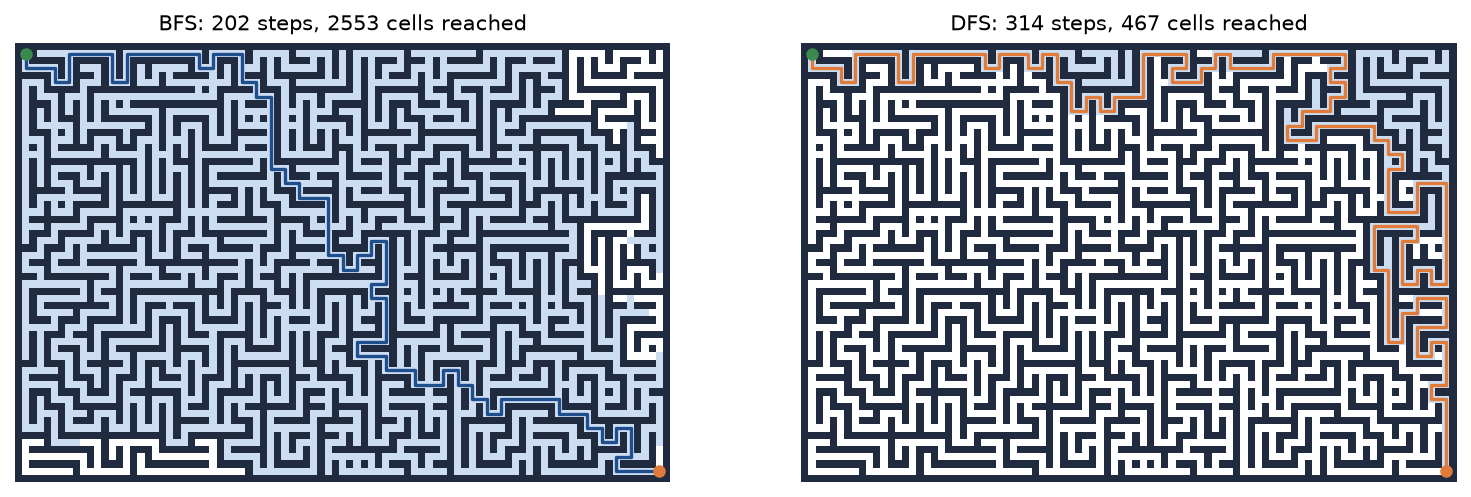
Two drawings of the same maze of 30 by 45 rooms with walls in dark blue. Left, BFS: almost every passage is shaded as reached, and a blue line marks a route of 202 steps from the top left to the bottom right. Right, DFS: only a band along the top and right is shaded, and an orange line marks a route of 314 steps that winds along the top edge and down the right side

BFS found the shortest route, 202 steps, after reaching 2553 cells; DFS found a route of 314 steps after reaching only 467. Over 40 mazes of the same size, DFS routes were 1.9190 times as long as BFS routes on average, from 1.1441 to 3.6857, and BFS reached 2678.7 cells on average against 698.8 for DFS: the shortest route costs a broad search, and DFS's luck in finding some route quickly comes with no guarantee about its length.

The second part solves word ladders: change one letter at a time, keeping a word at every step. The words come from the ENABLE list, a public-domain list of 172823 English words, which the project downloads once from a pinned commit of a public mirror into .data/graph-traversal/ at the repository root and checks against its SHA-256 digest before every use; the list contains many rare words, which the ladders show. Among the 3903 words of four letters, BFS turns cold into warm in 4 steps, cold, wold, word, ward, warm, after expanding 376 words, while DFS returns a ladder of 1767 steps. Black becomes white in 7 steps by BFS and in 3325 by DFS. The four-letter graph has 78 components; the largest holds 3807 words, and 65 words have no neighbour at all.

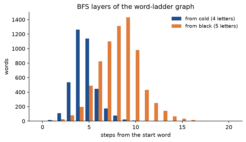
Bar chart of the number of words at each number of steps from the start word. From cold, among four-letter words, the counts rise to 1263 at four steps and fall to 1 at fourteen; from black, among five-letter words, they rise to 1431 at nine steps and fall to 1 at twenty

The layers of the word graph show why BFS works so well here: most words lie within a few steps of each other, so the answer is found in the first few layers, long before the search could reach the whole component. The default run, python graphs/graph-traversal/project/puzzle_solver.py, takes about two seconds. Options --rows, --columns, --gaps, --seed, --mazes and --pairs change the setup, --offline skips the word ladders, and --figures writes the PNGs elsewhere.

python graphs/graph-traversal/project/puzzle_solver.py
python graphs/graph-traversal/project/puzzle_solver.py --rows 60 --columns 80 --gaps 0.02 --pairs ape:man,wheat:bread

The notebook graph_traversal.ipynb follows this page: both searches traced on the worked graphs, the diagrams, bipartiteness, the stack search, implicit graphs, the counted costs and frontiers, the comparison with NetworkX and a short run of the project. The tests in tests check the worked example value by value, the invariants on hundreds of random graphs, the agreement with NetworkX and SciPy, the cost counts and every pitfall, and run in a few seconds:

python -m pytest graphs/graph-traversal

All graphs in the package, the examples and the tests are synthetic and generated from seeds. The only dataset is the ENABLE word list used by the project, which its authors placed in the public domain; it is downloaded at run time, verified by its SHA-256 digest and never committed.

In practice¶

NetworkX¶

NetworkX implements both searches in pure Python, iteratively, so recursion depth is never a problem. Built from the same edges in the same order, its graphs have the same adjacency lists as ours, and examples/compare_with_networkx.py shows that the two agree:

import networkx as nx

from graph_traversal import bfs, dfs, random_graph, to_networkx

graph = random_graph(200, 600, seed=1)
copy = to_networkx(graph)
order = bfs(graph, 0).order
assert order == [0, *(child for _, child in nx.bfs_edges(copy, 0))]
assert dfs(graph).preorder == list(nx.dfs_preorder_nodes(copy))
assert bfs(graph, 0).distance == nx.single_source_shortest_path_length(copy, 0)

On 300 random graphs, directed and undirected, the BFS order, the distances, the layers of nx.bfs_layers, the DFS preorder and postorder of nx.dfs_preorder_nodes and nx.dfs_postorder_nodes, and the verdicts of nx.is_bipartite and nx.find_cycle all agreed every time. The conventions that make results differ are worth knowing:

Neighbour order. Both libraries follow the order in which edges were added; bfs_edges, dfs_edges and the DFS node functions accept sort_neighbors to impose another. With neighbours sorted in reverse alphabetical order, NetworkX's DFS of the worked graph from oak visits oak, elm, fir, bay, yew, box, fig, ivy, gum, ash.
Shortest paths. Without weights, nx.shortest_path runs a bidirectional BFS, growing one search from each end. It always finds a fewest-edge path, but among several it may choose a different one from a single BFS: on random graphs with 60 vertices it returned another path of the same length in 250 of 1754 cases.
Edge labels. nx.dfs_labeled_edges labels a tree edge "forward", which is not the forward edge of the classification above, lumps back, forward and cross edges together as "nontree", and adds "reverse" events when the search steps back along a tree edge. The classes have to be recovered from the times.
Early exit. nx.generic_bfs_edges stops as soon as every vertex has been seen, so it can skip the last adjacency lists: on the worked graph it read 23 entries against our 26. It also takes a neighbour function, which is how CountedNeighbours counts its work.
Deprecations. nx.bfs_predecessors is deprecated in NetworkX 3.7; the parents are the tree edges of nx.bfs_edges.

In wall-clock time NetworkX and the package are about equally fast, both being plain Python: in repeated runs of the example NetworkX took between about 0.8 and 1.1 times as long as bfs on a graph with 20000 vertices and 100000 edges.

SciPy¶

scipy.sparse.csgraph.breadth_first_order and depth_first_order run in compiled code on a sparse matrix whose rows are vertex indices, 15 to 25 times faster than the package on the same graph in repeated runs, once the matrix is built. They return valid orders, and the depth-first one is a true depth-first order, but they take each vertex's neighbours in the order the sparse matrix stores them, which for an undirected graph built from one half of the matrix is not the order of insertion: on the worked graph its depth-first order from oak is oak, ash, fir, bay, gum, fig, ivy, box, elm, yew. Compare sets, distances and validity with SciPy, not sequences. For large numerical graphs, connected components and shortest paths over millions of edges, it is the tool of choice.

Elsewhere¶

The Boost Graph Library in C++ exposes both searches through visitor objects with callbacks for each event (discover vertex, examine edge, tree edge, back edge, forward or cross edge, finish vertex), which is exactly the event list of trace.py; JGraphT in Java offers them as iterators. Garbage collectors traverse the graph of live objects: the mark phase of a mark-and-sweep collector is a graph search from the roots, often depth-first with an explicit mark stack, and Cheney's copying collector is a breadth-first search whose queue is the copied objects themselves. Web crawlers search the link graph breadth-first so that pages close to the seeds come first. Flood fill in image editors, connected-component labelling in vision, puzzle solvers, package managers resolving dependencies and compilers detecting cycles among modules are all traversals. Version control systems answer "is this commit an ancestor of that one?" by graph search on the commit graph, and routing algorithms such as Dijkstra's and A* are BFS with a priority queue for a frontier.

When to use which:

Use BFS for fewest-edge paths, distances in steps, layers, nearest-source questions and bipartiteness.
Use DFS for cycle detection, topological order, strongly connected components, bridges and articulation points, and anything that needs discovery and finish times or edge classes.
Use either for plain reachability and connected components; DFS needs no queue, BFS no recursion.
Use Dijkstra's algorithm, not BFS, when edges have weights, and 0-1 BFS when the weights are only 0 and 1.
In Python, use the iterative DFS or a library for anything that may be deep, and NetworkX or SciPy for large graphs.

Pitfalls¶

Marking a vertex when it leaves the queue instead of when it enters. The order and distances stay right, but a vertex already waiting is enqueued again by every later neighbour: on a random graph with 30 vertices and 300 edges the queue received 301 entries instead of 30. examples/common_mistakes.py runs this and every following mistake.
Using a Python list as the queue. list.pop(0) moves every remaining item, so BFS from the centre of a star with 3000 vertices moved 4495501 items; collections.deque moves none.
Reading a weighted path off BFS. BFS minimises edges, not weight: on the road map it returns home, park, work of weight 9 while home, mill, farm, port, work weighs 7. Use Dijkstra's algorithm, or 0-1 BFS for weights 0 and 1.
Changing a vertex's parent or distance when it is reached again. In BFS the first discovery is final; when elm is dequeued in the worked example, fir is already queued and keeps parent ash.
Forgetting the marks, or setting them too late. Without marks a depth-first search follows every path, and on a chain of k diamonds it enters 2^(k + 2) − 3 vertices, 131069 for 15 diamonds with 46 vertices:

E of k equals 3 plus 2 times E of k minus 1, with E of 0 equal to 1, so E of k equals 2 to the k plus 2, minus 3

Marking only when a vertex is finished stops repetition on a DAG but loops for ever on any cycle, and in an undirected graph every edge is one: the search walks back and forth along its first edge. - Treating the stack search that marks on push as DFS. It reaches every vertex, but its order is often not depth-first, its tree is not a depth-first tree, and it has no finish times, so cycle detection, topological sorting and edge classification built on it give wrong answers. Use recursion, the iterator stack or mark on pop. - Calling an edge to a finished vertex a cross edge without comparing discovery times. If the finished vertex was discovered after the current one it is a descendant and the edge is a forward edge; on the worked graph that mistake turns 1 forward and 3 cross edges into 0 and 4. - Detecting cycles with the wrong notion of seen. In a directed graph only an edge to a gray vertex closes a cycle; an edge to any visited vertex also catches forward and cross edges and calls a diamond cyclic. In an undirected graph the edge back to the parent is not a cycle; counting it calls every tree cyclic. - Testing bipartiteness from one vertex only. Every component needs its own start, or an odd cycle elsewhere, such as a triangle after a path, goes unnoticed. - Relying on IndexError at the edge of a grid. Python reads index −1 as the last row or column, so a move off the top wraps round to the bottom; on the worked maze the broken neighbour function gave S a path of 2 steps to T instead of 12. Test the bounds explicitly. - Recursing on large graphs. Recursive DFS fails beyond about a thousand vertices on one path; use the iterative version rather than raising the recursion limit. - Expecting a particular order from another implementation. Visit orders depend on neighbour order and on the algorithm's details, bidirectional search or storage order included; compare distances, reachable sets and validity, not sequences, unless both sides fix the order.