Recurrences and the master theorem

A recursive function's cost is defined in terms of itself: merge sort costs two half-size sorts plus a merge, binary search one half-size search plus one comparison, a naive Fibonacci call two smaller calls plus an addition. A recurrence writes that self-reference down, and solving it turns it into a closed form or a growth class such as Θ(n log n). This page reads recurrences off real code, solves them by unrolling, by recursion trees and by the substitution method, states the master theorem in its common form and in the extended form with logarithmic factors, gives the matching rule for decreasing recurrences such as T(n) = 2T(n − 1) + n², shows by simulation where these theorems stop applying, explains why floors and ceilings do not change the answer, solves linear recurrences by their characteristic roots with the Fibonacci numbers and Lamé's theorem as examples, and points to the Akra-Bazzi method for uneven splits. Every answer is checked against exact values computed from the definition and against operations counted in running code. Afterwards you will be able to write the recurrence of a recursive function, pick the method that solves it, avoid the habits that give wrong answers, and confirm the answer by counting. It builds on Asymptotic analysis and Recursion, and the tools are used throughout Merge sort, Quicksort and Divide and conquer.

The solvers, the evaluator and the instrumented functions need only the standard library; to run the plots and the notebook install the base group, and the graphs group for the comparison with SciPy's root finder.

Intuition

Picture a large job handed down an organisation. The person at the top splits it into a few parts, gives each part to an assistant, and does some coordinating work of their own: reading the brief, merging the results. Each assistant does the same with their part, and so on down to people who handle a part so small that they just do it. The total effort is the sum of everybody's own work, and the only question is where most of it sits. If coordinating is expensive and the parts shrink fast, the person at the top does most of the work. If every layer of the organisation does the same amount in total, the total is that amount times the number of layers. If the job multiplies into very many tiny parts, the crowd at the bottom does most of the work, however cheap each part is.

A recurrence is that organisation chart written as an equation, and every method on this page is a way of adding up the chart without drawing all of it.

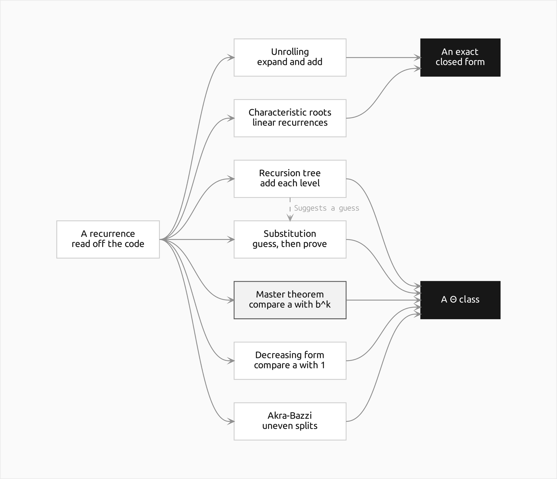
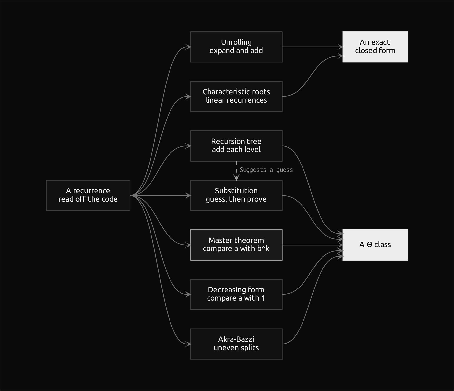
The diagram shows the route this page follows. Code gives a recurrence; unrolling and characteristic roots give an exact closed form; the recursion tree, the substitution method, the master theorem (highlighted), its decreasing form and Akra-Bazzi give a Θ class; and every answer, one of the two filled boxes, is checked by computing the recurrence exactly and by counting operations in the code.

How it works

From code to a recurrence

The cost T(n) of a recursive function on an input of size n is the work the call does itself plus the cost of each recursive call it makes. Three things have to be read off the code: how many recursive calls a call makes, the size of the input each one gets, and how much work happens outside the recursive calls, called the driving function f(n). The base case, where the function returns without recursing, gives the starting values. Most divide-and-conquer code has the shape below, with a subproblems, each a fraction 1/b of the input:

Code that peels off a constant amount each time, such as recursion on the rest of a list, has a decreasing shape instead:

The functions in programs.py, multiplication.py and fibonacci.py count their own operations, and their recurrences read as follows:

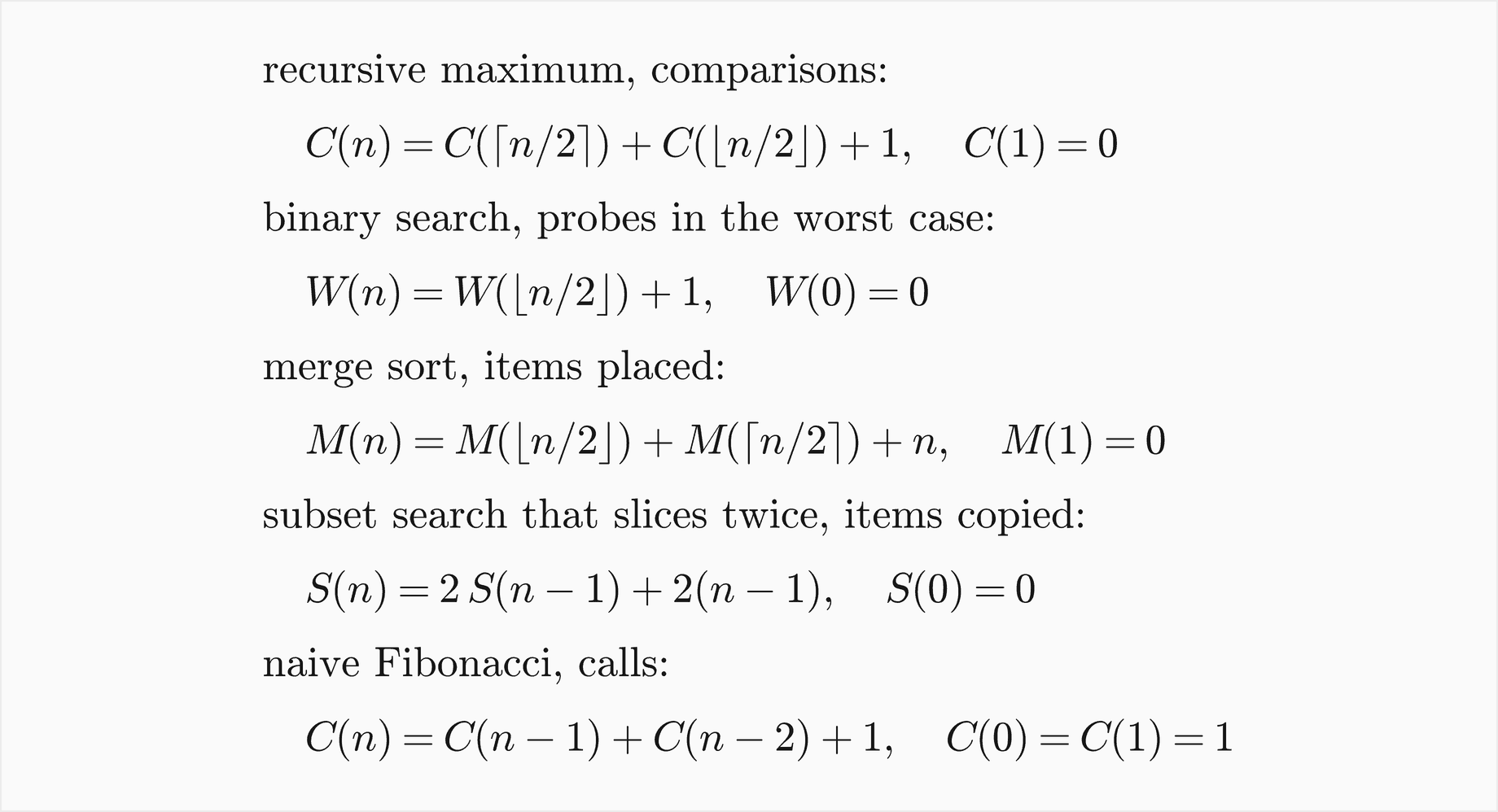
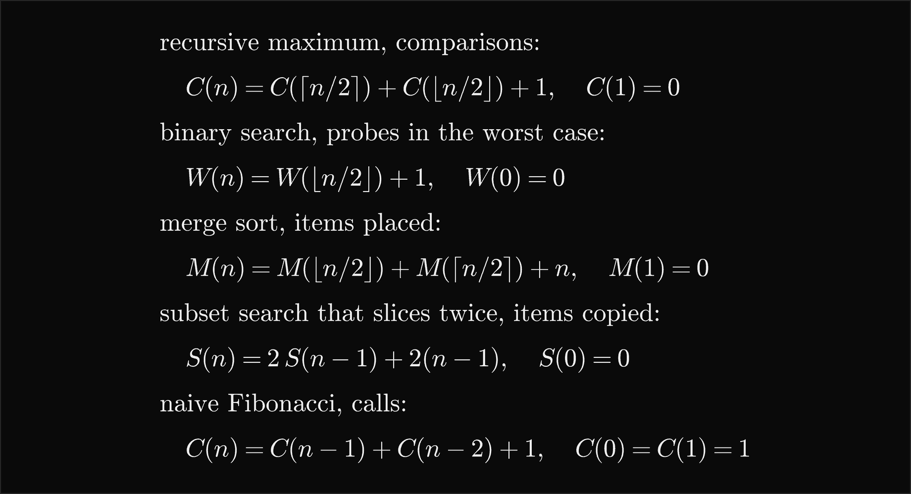
Each line comes from one look at the code. The recursive maximum finds the largest item of each half and compares the two answers once. Binary search compares the middle item once and continues in at most ⌊n/2⌋ items. Merge sort sorts both halves and then places all n items into the merged list. The subset search counts the subsets of n items with a given total by trying the first item in and out, and hands each of its two recursive calls its own slice items[1:]; each slice copies the other n − 1 items, so a call copies 2(n − 1) items, a linear cost hidden in an expression written twice. The naive Fibonacci function calls itself on n − 1 and n − 2 and adds the results.

Three habits make the reading reliable. Count what the code does, not the lines it has: a slice, a string concatenation or x in some_list costs time proportional to its length. Write the argument of each recursive call exactly, with its floor or ceiling, because only then can the recurrence be checked against the code; the floors can be dropped later, for the reason given below. And decide what is being counted, comparisons, items moved or calls, since the same function has a different recurrence for each, and the tests compare each recurrence with the matching counter.

Unrolling

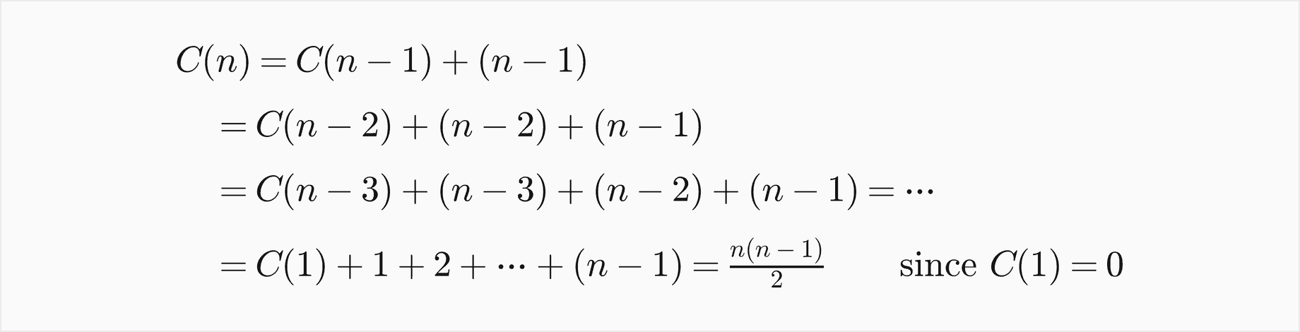
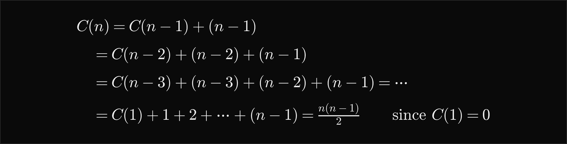
Unrolling, also called back substitution or iteration, replaces T on the right-hand side by its own definition again and again until only the base case is left, then adds up the terms. Selection sort written recursively finds the largest of n items with n − 1 comparisons and sorts the rest, so C(n) = C(n − 1) + n − 1 with C(1) = 0, and the terms form an arithmetic sum:

For a halving recurrence, such as the worst case of binary search on n = 2^L items, the argument reaches 1 after log2 n steps:

The general dividing recurrence unrolls into one term per level, with a^i copies of f at size n/b^i on level i, and the base cases a^L T(1) at the bottom, L = log_b n levels down:

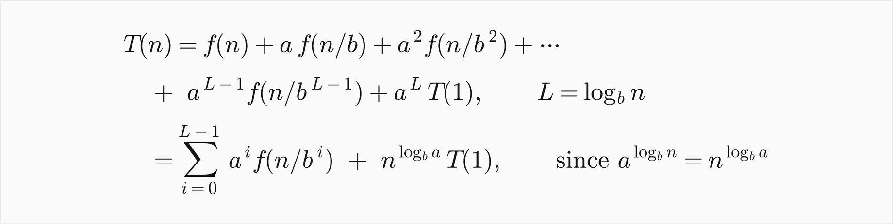
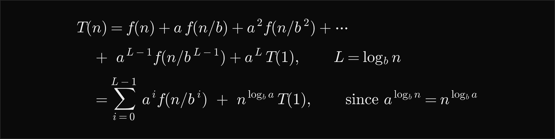
The identity at the end is worth remembering: the number of base cases is n^(log_b a), the critical power that the master theorem compares f with. Unrolling is exact, so it gives closed forms such as 3n^(log2 3) − 2n for T(n) = 3T(n/2) + n, and every closed form in the package's CLOSED_FORMS list is checked against values computed from the definition by exact.evaluate, which follows the recurrence with a memo table and an explicit stack rather than Python recursion.

Recursion trees

A recursion tree draws unrolling as a tree. Each node is one call, labelled with the work it does itself; its children are the calls it makes. Adding the costs level by level gives the same terms as unrolling, laid out so that one can see where the work is. The three trees below differ only in f(n), and each sits at one end of the possibilities.

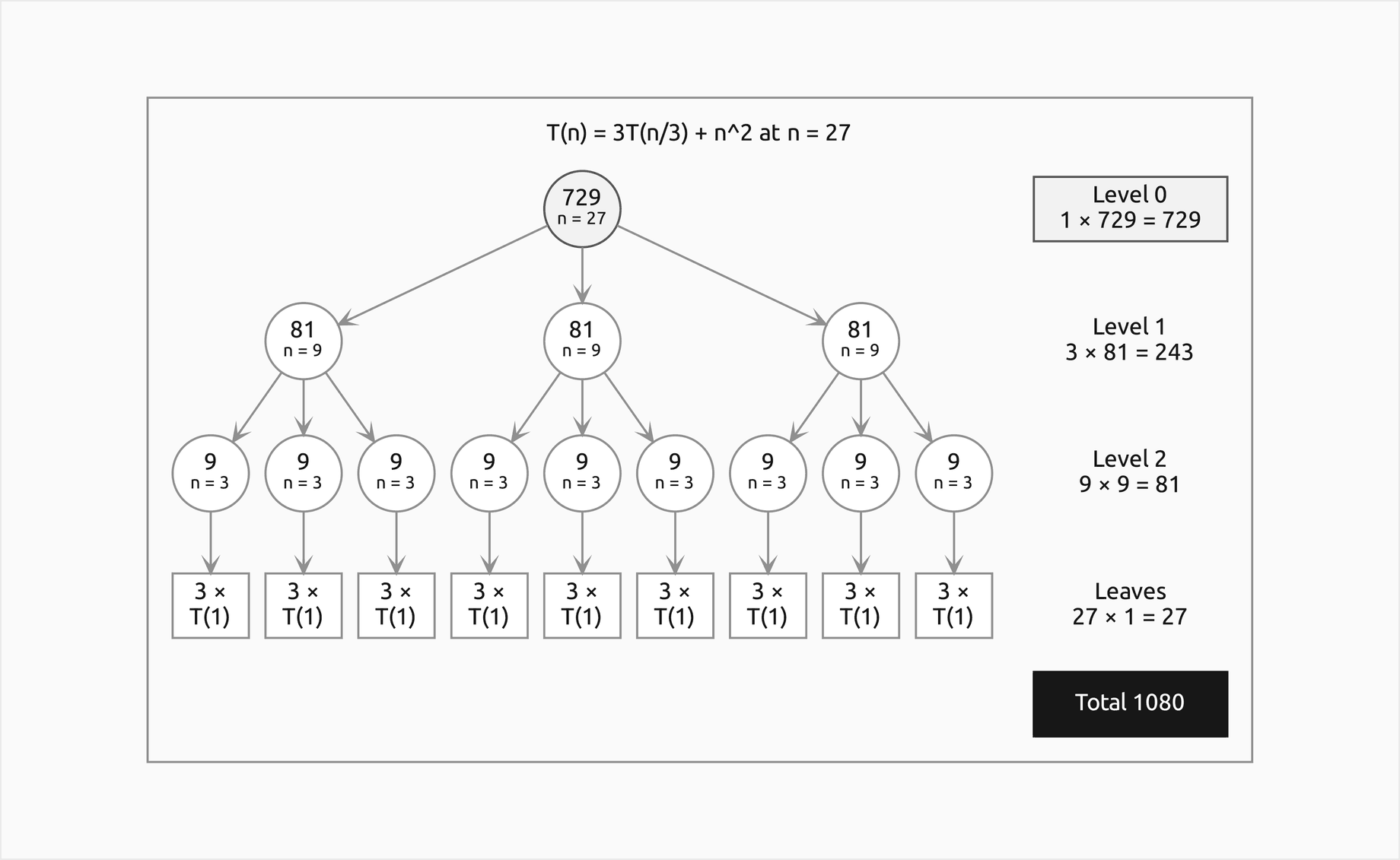
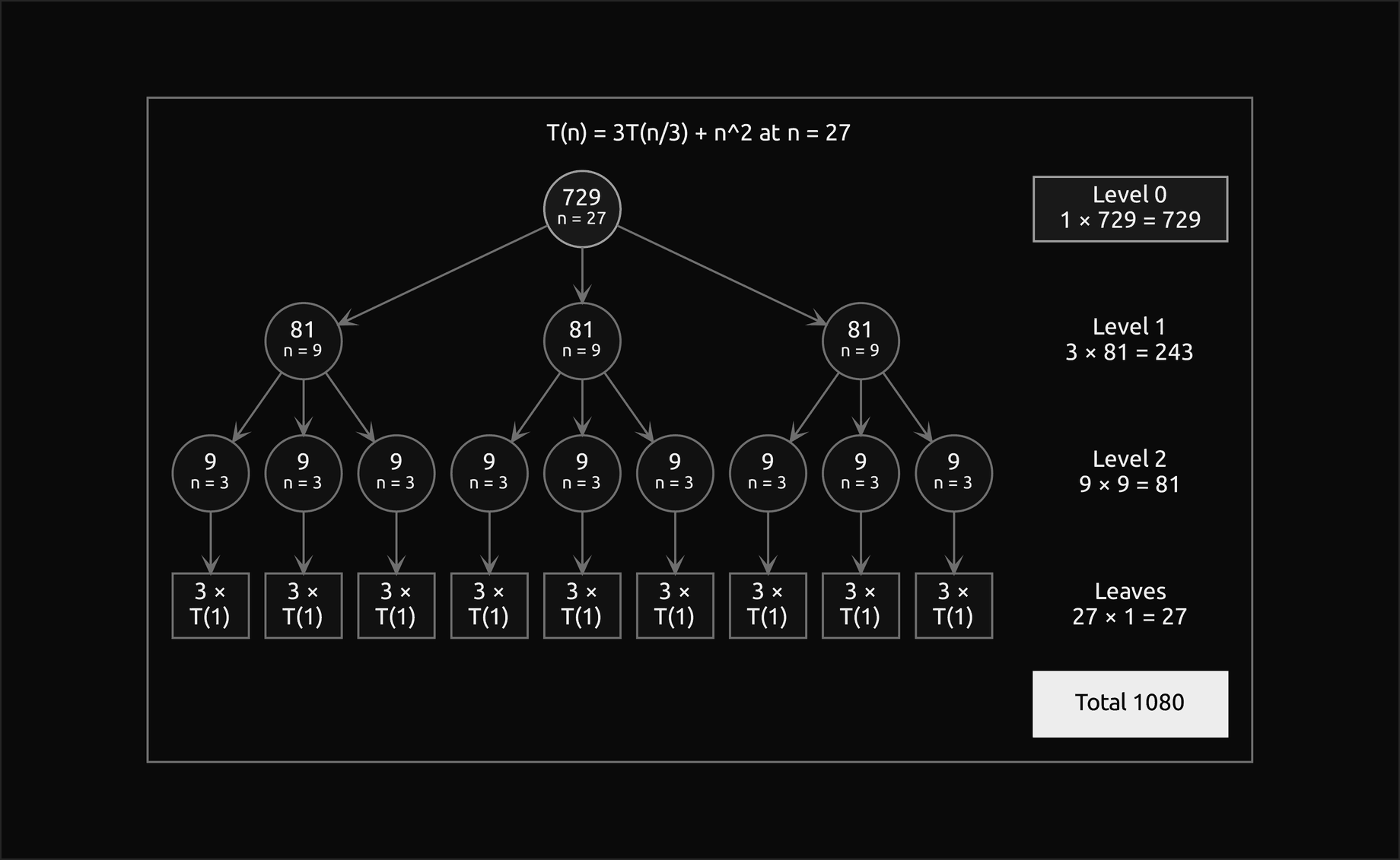
With f(n) = n², each node costs the square of its size and there are only three times as many nodes on the next level, so each level costs a third of the one above: 729, 243, 81 and 27. The sum is less than one and a half times the root's cost, and the root dominates.

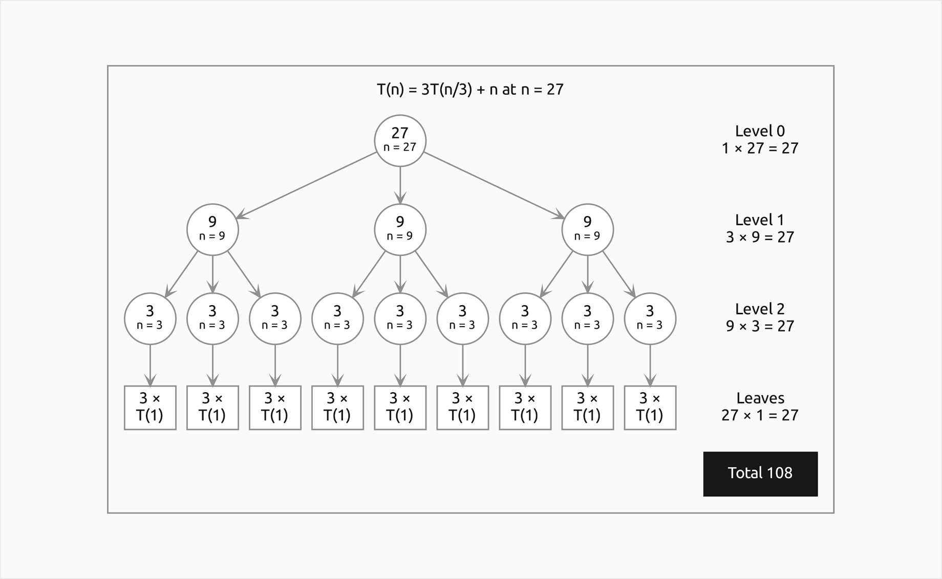
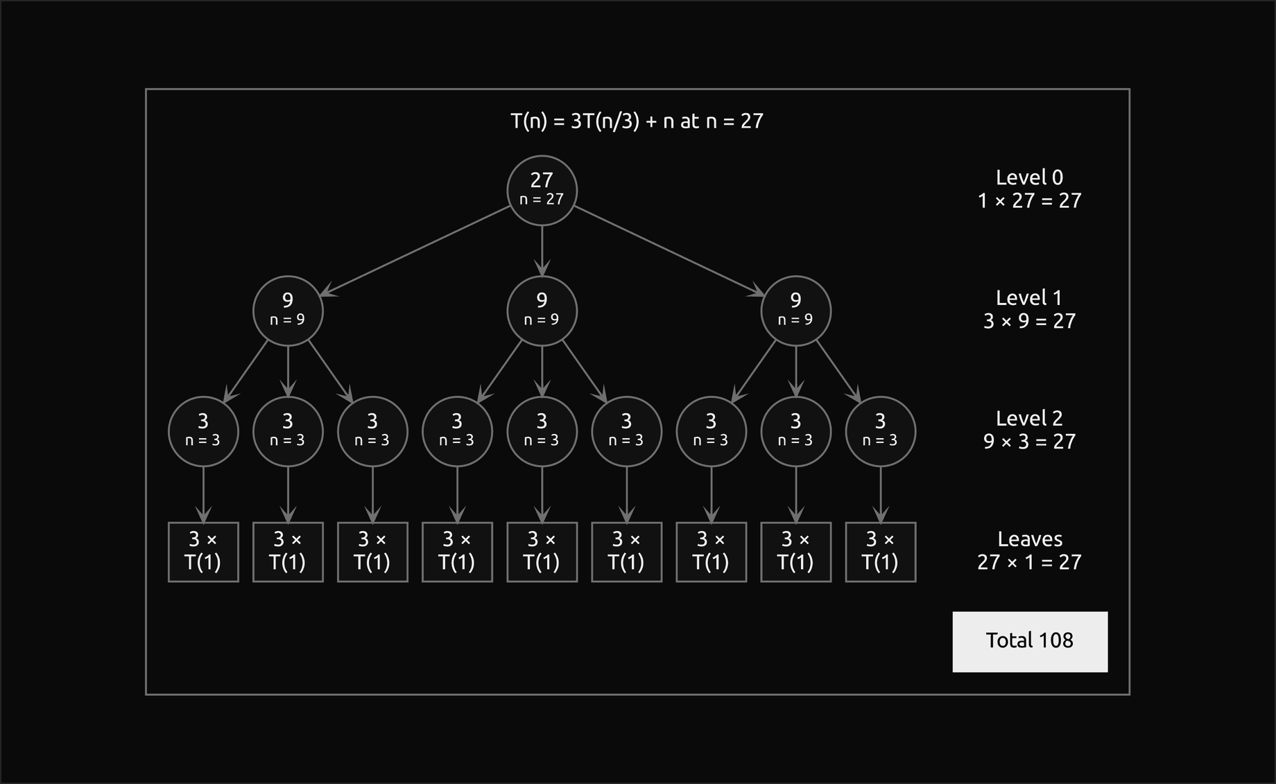
With f(n) = n, tripling the nodes exactly cancels dividing their cost by three, so every level costs n, and the total is n times the number of levels, n(log3 n + 1).

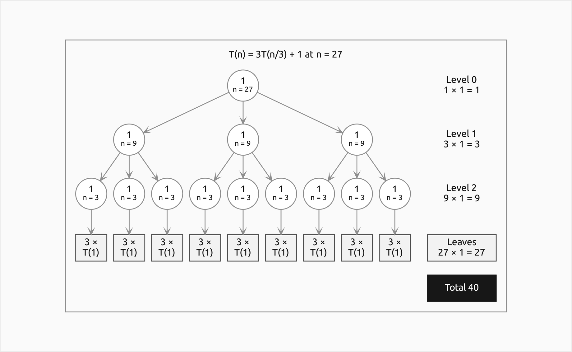
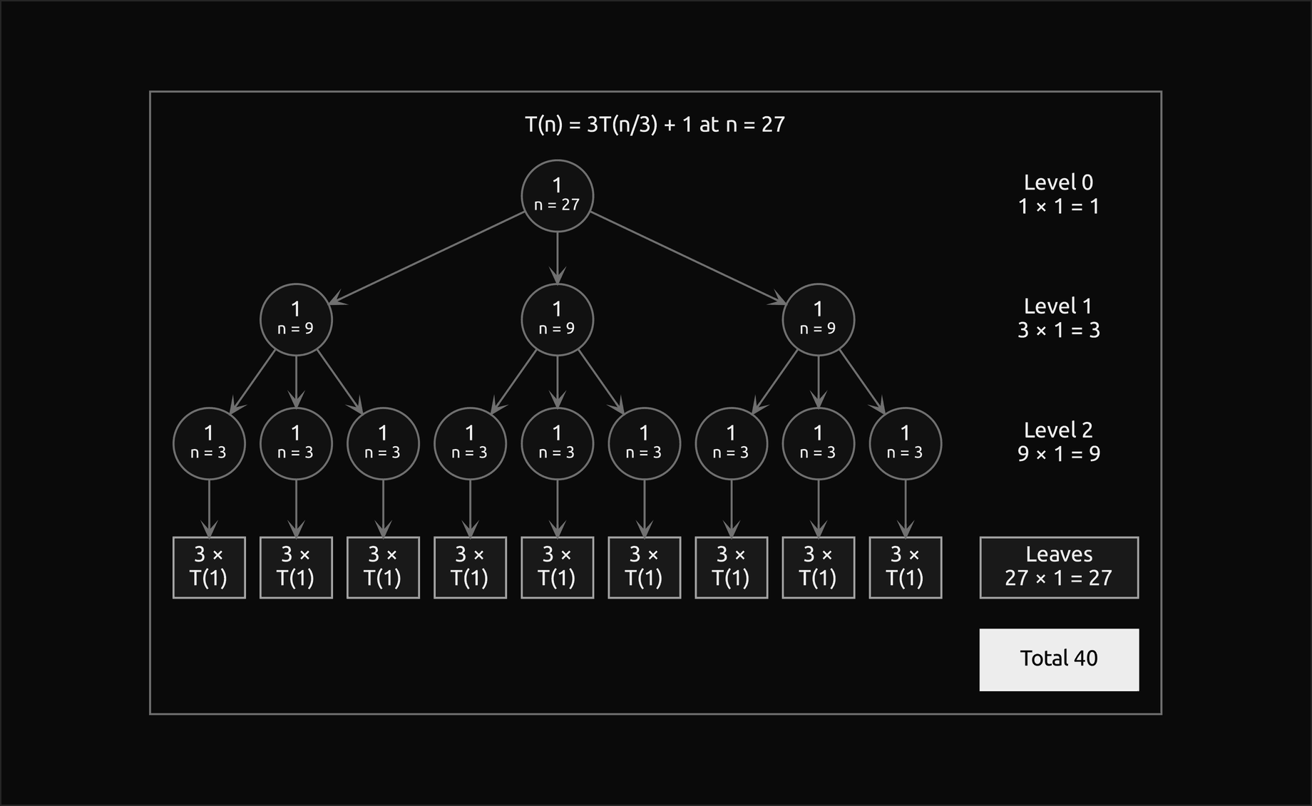
With f(n) = 1, each level costs three times the one above, and the twenty-seven leaves alone cost more than all the levels above them together. The leaves dominate, and their number, n^(log_b a) = n here, sets the answer.

A decreasing recurrence gives a tall tree. For T(n) = 2T(n − 1) + n² the tree has n levels, level i holds 2^i calls of size n − i, and the level costs 2^i(n − i)² grow towards the bottom until the shrinking factor (n − i)² takes over a few levels above the leaves, as the worked example draws.

The substitution method

The substitution method guesses the answer and proves it by induction: assume the bound for every argument smaller than n, put it into the right-hand side of the recurrence, and show that the bound comes back for n with the same constant. The base cases must hold too. The recursion tree is a good source of guesses, and induction turns them into proofs; substitution.py carries out the inductive step with numbers, so a step that fails shows the n where it fails.

The method has a well-known trap. The recursive maximum makes C(n) = n − 1 comparisons, so C(n) ≤ cn is true with c = 1. Yet the induction for that bound does not go through:

The step leaves a + 1 behind at every n, and no choice of c removes it, because the + 1 does not grow with n while the hypothesis has no room to absorb it. Increasing c does not help. The fix is to prove something stronger: subtract a lower-order term from the guess. The stronger hypothesis is used twice on the right-hand side, so it pays the extra 1:

Proving a stronger statement is easier here because the induction hypothesis is stronger too. The same move fixes the worked example below, where the guess c n^(log2 3) fails by n at every step and c n^(log2 3) − dn succeeds for d ≥ 2.

The opposite mistake looks like a proof and is not one: assuming M(n/2) ≤ cn/2 for merge sort's placements M(n) = 2M(n/2) + n gives M(n) ≤ cn + n, and declaring that "O(n)" changes the constant from c to c + 1 at every level, which proves nothing. The bound M(n) ≤ 10n is in fact false from n = 2^11 on, since M(n) = n log2 n when M(1) = 0, and common_mistakes.py shows the overshoot at n = 2^12.

The master theorem

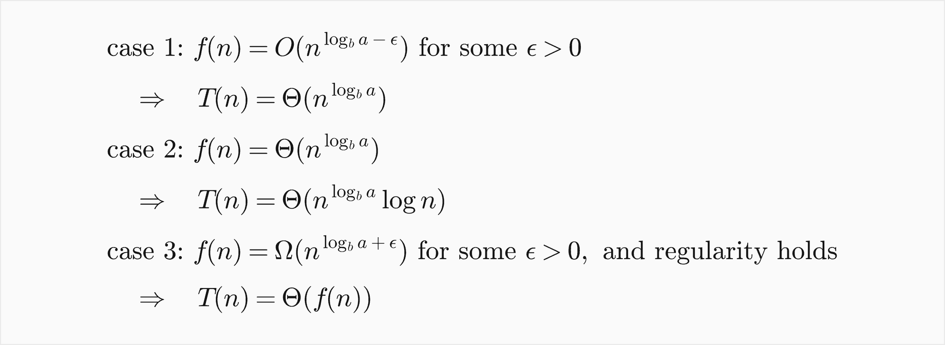
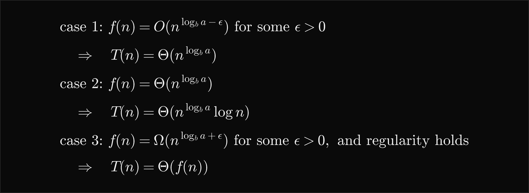
The master theorem solves T(n) = aT(n/b) + f(n) by comparing f(n) with n^(log_b a), the cost of the leaves, whose exponent log_b a is called the critical exponent. In its common form:

Case 3 needs one more condition, regularity, which says that the work shrinks by a constant factor from each level to the next:

The constant c must be strictly below 1 and must not depend on n, and the inequality needs to hold only from some n on. For polynomial f regularity is automatic: with f(n) = n^k it reads a/b^k ≤ c, which is exactly the case 3 condition. It matters for driving functions that jump around, as the section on failures shows.

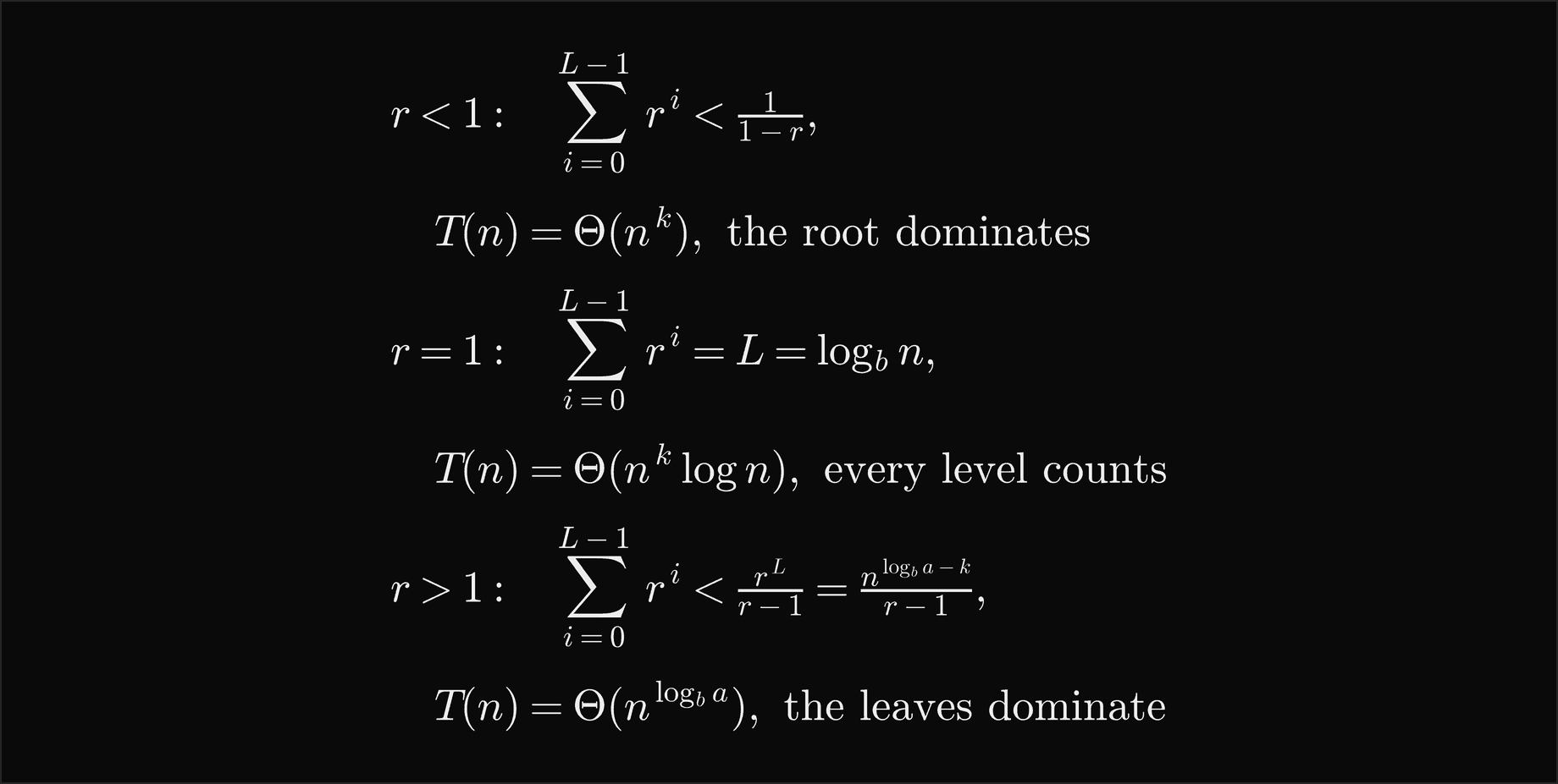
The cases are the three trees above. For f(n) = c n^k, level i costs c n^k times r^i with r = a/b^k, a geometric series, and the sum depends only on whether r is below, equal to or above 1. Case 1 is r > 1, where the leaves win; case 2 is r = 1, where every level counts; case 3 is r < 1, where the root wins. The cost section works the series out.

Between the cases there are gaps. With f(n) = n log n and n^(log_b a) = n, f is larger than n, but not by a factor n^ε for any ε > 0, so neither case 2 nor case 3 applies and the common form says nothing; the same happens for n²/log n against n². The ε in cases 1 and 3 means "polynomially smaller" and "polynomially larger", and logarithms are neither.

The extended form with logarithmic factors

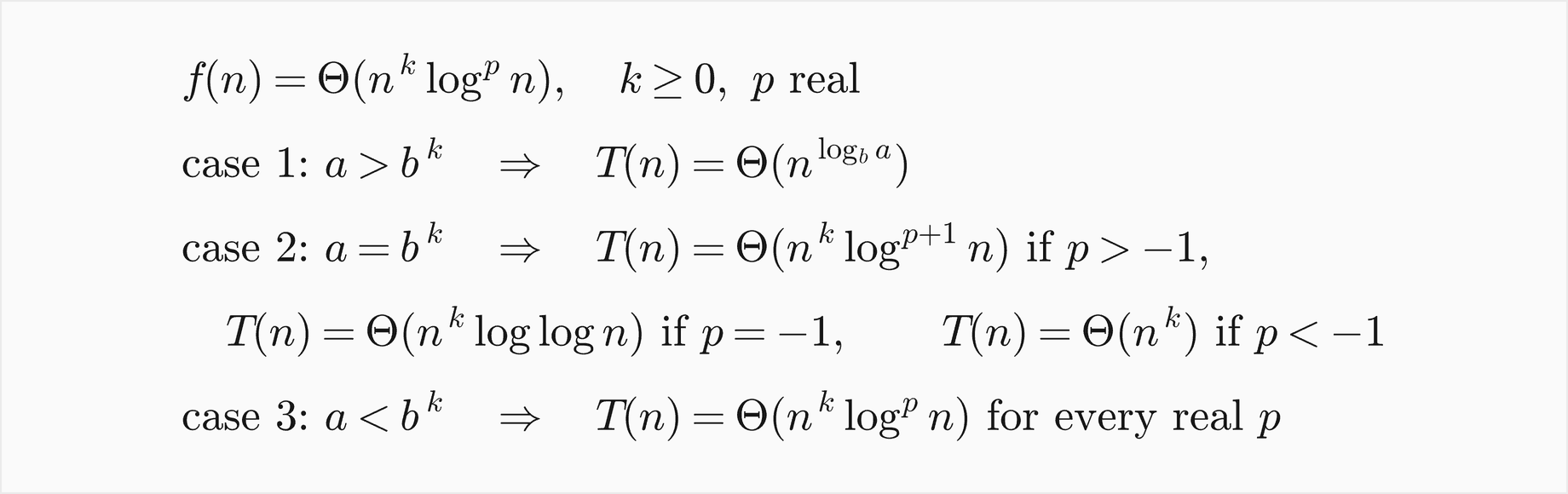
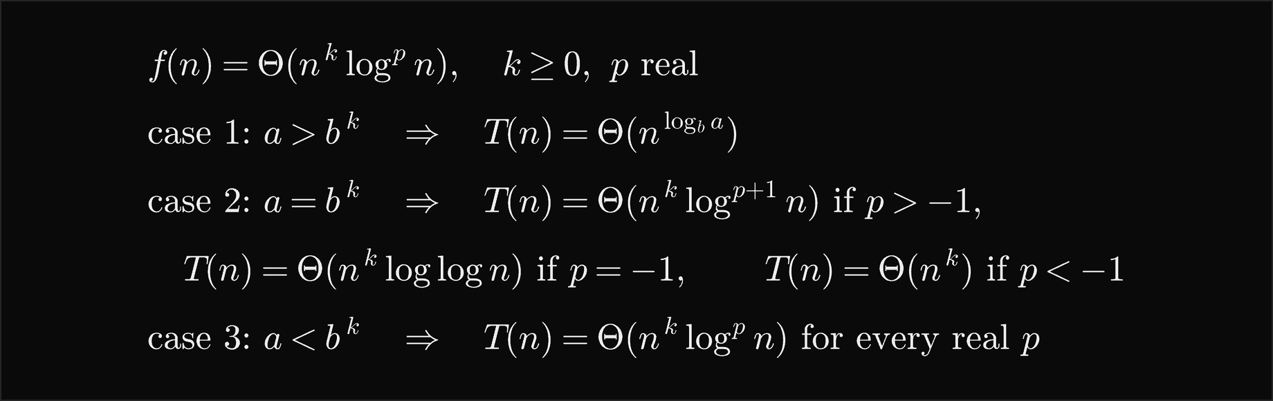
Most driving functions in practice have the form n^k log^p n, and for those the gaps can be closed. Comparing a with b^k is the same as comparing log_b a with k:

Case 2 is where the logarithms matter. When a = b^k every level has the same polynomial part, and the logarithm is all that varies: level i costs n^k times (log b)^p (L − i)^p, so the total is n^k times a sum of j^p:

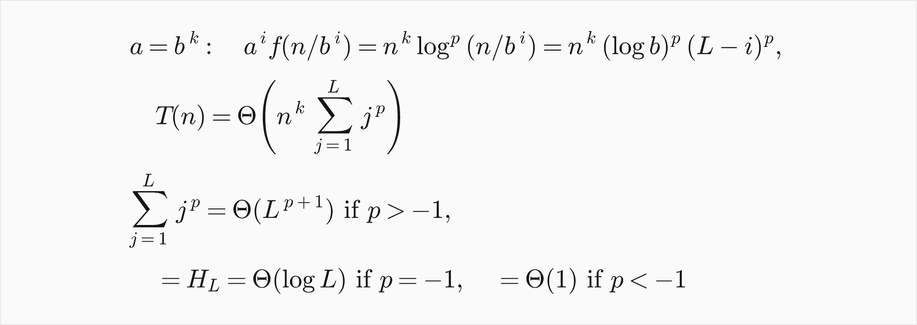
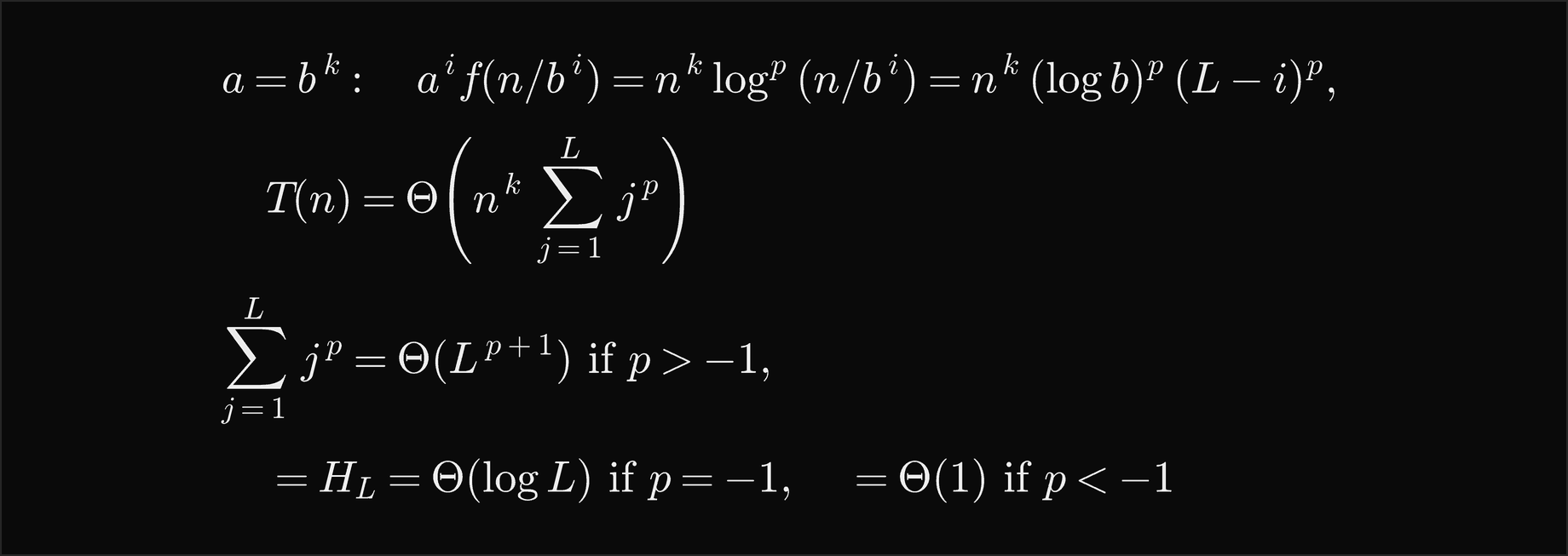
With L = log_b n that gives the three sub-cases: an extra log^(p+1) n, an extra log log n, or nothing. In case 3 the root's term dominates for every p, so the answer keeps the factor log^p n even when p is negative. A frequently quoted version of the theorem says Θ(n^k) for case 3 with p < 0; that is only an upper bound. For T(n) = 2T(n/4) + n/log n the answer is Θ(n/log n), and T(n)/n falls steadily towards 0 (from 0.1168 at n = 4^10 to 0.0346 at n = 4^30), so Θ(n) is wrong.

The solver in master.py prints exactly these steps. For T(n) = 5T(n/2) + n² it reports a = 5, b = 2, the critical exponent log_2 5 = 2.3219, f(n) = n² with k = 2 and p = 0, the comparison a = 5 > b^k = 4, case 1 and the answer Θ(n^2.3219). Its common-form solver refuses the three examples with a logarithmic gap and agrees with the extended form on every recurrence where both apply, which the tests check on 300 random recurrences.

Decreasing recurrences

For T(n) = aT(n − b) + f(n) the tree has about n/b levels and a^i nodes on level i, so the comparison is between a and 1, and the size of each node shrinks only by b per level:

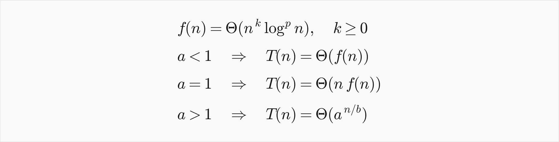
The case a > 1 deserves care. The number of nodes, about a^(n/b), multiplied by the cost of the most expensive node, about n^k, gives the bound O(n^k a^(n/b)), which is true but never tight when k > 0. The level costs grow geometrically towards the leaves while the node costs shrink, and the series converges:

So T(n) is a constant times a^n. For T(n) = 2T(n − 1) + n² the constant is the sum of j²/2^j, which is 6, and the exact solution is 6 · 2^n − n² − 4n − 6: the n² 2^n of the loose bound never appears. Towers of Hanoi, with f(n) = 1, makes 2^n − 1 moves, and the subset search, with f(n) = 2(n − 1), copies 2^(n+1) − 2n − 2 items: copying the remaining items at every call costs a constant factor, not a factor n, because most calls are near the leaves where little is left to copy. At n = 60 the loose bound n² 2^n is 600 times the true value, and the gap keeps growing.

When the theorem does not apply

The master theorem has hypotheses: a constant a ≥ 1, a constant b > 1, a positive driving function, and for case 3 regularity. Each failure below is evaluated exactly by failures.py and drawn in figures/failures.png.

• A non-constant a. T(n) = nT(n/2) + n multiplies n, n/2, n/4 and so on together, so log2 T(2^L) is about L(L + 1)/2: at n = 2^24 it is 301.4014. Putting a = n into n^(log_b a) would claim n^(log2 n), whose logarithm is L² = 576. The truth is not a polynomial at all, and the misapplied formula is off by a factor of two in the exponent.
• A fraction a < 1. T(n) = (3/4)T(n/2) + n has fewer than one subproblem per call, which no algorithm has. The root dominates even more strongly than in case 3, T(n)/n tends to 1/(1 − 3/8) = 1.6, and T(n) = Θ(f(n)) by direct summation, not by the theorem; the formula n^(log_b a) = n^(−0.4150) would be a decreasing function.
• A negative driving function. T(n) = 8T(n/2) − n³ with T(1) = 1 gives T(n)/n³ = 1 − log2 n exactly, so T(4) = −64 and the values stay negative. Reading off a = 8, b = 2, k = 3 would suggest case 2 and Θ(n³ log n), a "running time" with the wrong sign.
• A logarithmic gap. T(n) = 4T(n/2) + n²/log n is n²(H_L + 1) exactly, with H_L the harmonic number of L = log2 n: at n = 2^40, T(n)/n² = 5.2785 and still growing, while T(n)/(n² log2 n) = 0.1320 and still falling. The common form has no case for it; the extended form's case 2b gives Θ(n² log log n).
• Broken regularity. With T(n) = T(n/2) + f(n), where f(n) = n² on even levels L = log2 n and n on odd ones, f is polynomially larger than n^(log_2 1) = 1, yet case 3's answer Θ(f(n)) is wrong: at odd levels T(n) ≥ f(n/2) = n²/4, and T(n)/f(n) is 143165577.8667 at n = 2^29. The answer is Θ(n²).

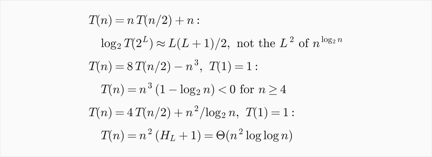
The three closed forms come from unrolling and are exact; the simulation draws each of them next to the claim a careless reading would make.

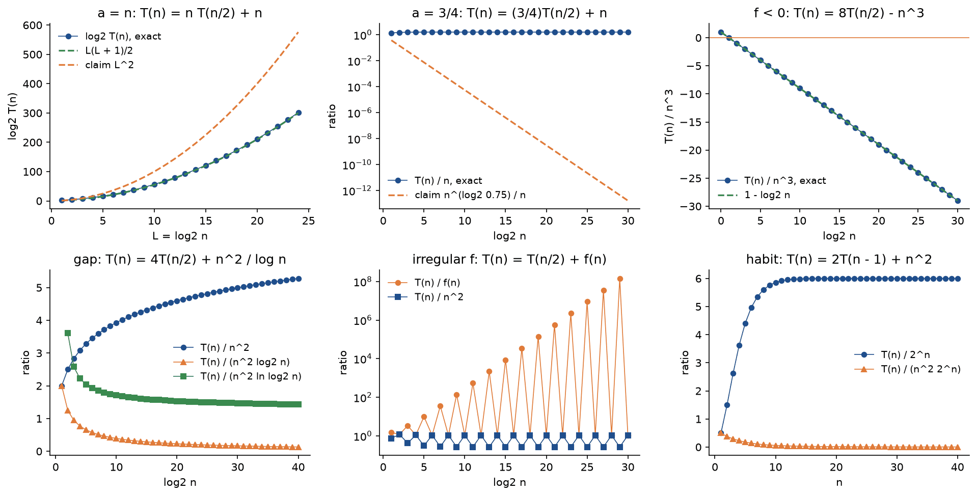
Each panel divides the exact values by a candidate answer. A flat line means the candidate has the right growth; a line that keeps rising or falling means it does not. The last panel is the decreasing habit from the previous section: T(n)/2^n settles at 6, and T(n)/(n² 2^n) falls like 6/n².

Floors, ceilings and sizes between powers

Real code splits n items into ⌈n/2⌉ and ⌊n/2⌋, and n is rarely a power of 2. The clean recurrence on powers of b gives the right Θ class anyway, for a short reason: the recurrences used here are non-decreasing in n, so T(n) is caught between its values at the powers of b on either side, and those two differ by at most a constant factor whenever the answer is a polynomial times a power of a logarithm.

Sometimes the floors can even be solved exactly. The most comparisons merge sort can make satisfy a recurrence with both a ceiling and a floor, and its closed form holds for every n:

The tests check it for every n below 3000, and floors.py checks that merge sort's placements M(n) = 2M(n/2) + n with M(1) = 0, written with floors, with ceilings and with the split the code makes, are non-decreasing and sandwiched between neighbouring powers of two.

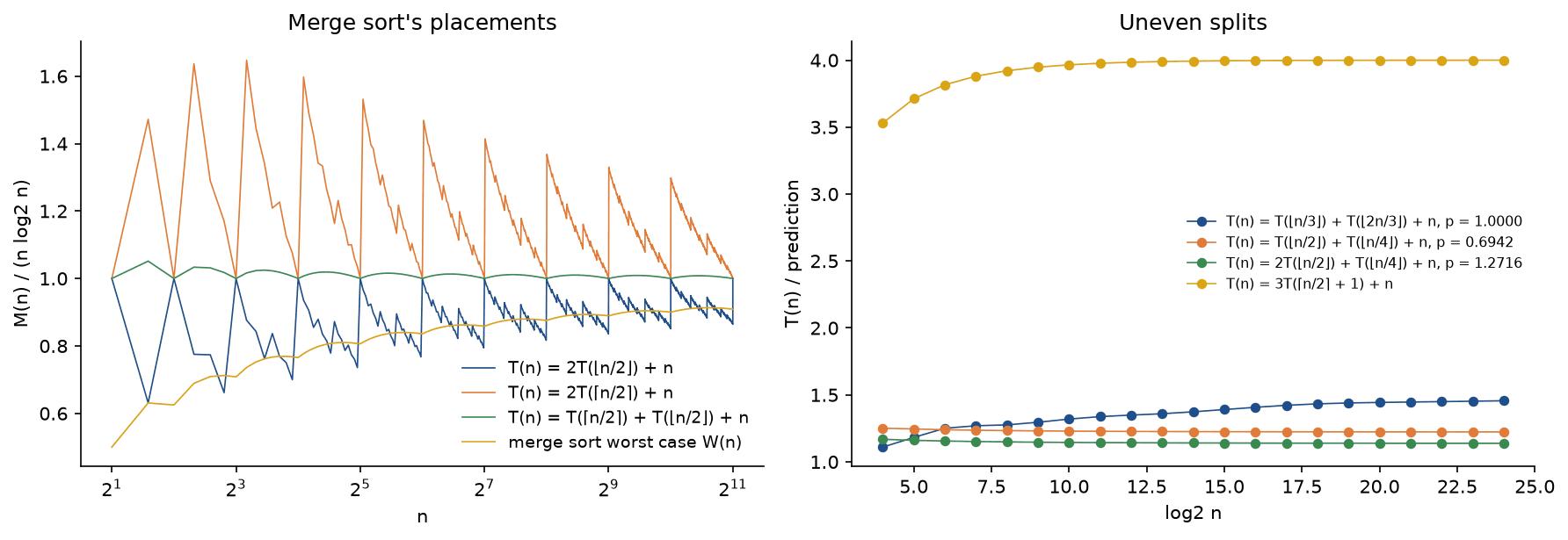
The saw-tooth on the left is the effect of rounding: just above a power of two the ceiling version pays for a nearly empty extra level, and at n = 1500 the three versions give M(n)/(n log2 n) = 0.8935 (floor), 1.0871 (ceiling) and 1.0080 (split). The ratios stay within constant bounds and narrow as n grows. The right panel shows that even arguments shifted by a constant, ⌈n/2⌉ + 1 as in Karatsuba's original sum form, keep the exponent log2 3.

Linear recurrences and characteristic roots

Some recurrences are not divide and conquer at all but linear combinations of the previous few terms, with constant coefficients. Fibonacci numbers, tilings, paths in small automata and the call count of naive Fibonacci are of this kind. Trying a_n = x^n turns the recurrence into a polynomial equation, the characteristic equation:

Every root r gives a solution r^n, and because the recurrence is linear, sums of solutions are solutions. A root of multiplicity m contributes r^n, n r^n, up to n^(m−1) r^n, and the d initial values fix the d weights:

roots.py finds integer roots exactly by trying the divisors of the constant term and the rest with the quadratic formula or the Durand-Kerner iteration, and linear.py solves for the weights by Gaussian elimination. The growth is set by the largest root that carries a weight: Θ(4^n) for roots 4 and −3, Θ(n 6^n) for a double root 6, and Θ(1) for complex roots on the unit circle, which make the sequence periodic. A constant term s adds the constant particular solution s/(1 − c_1 − ... − c_d), unless 1 is itself a root.

Fibonacci numbers and Lamé's theorem

The Fibonacci recurrence F(n) = F(n − 1) + F(n − 2), F(0) = 0, F(1) = 1 has the characteristic equation x² = x + 1 with roots φ and ψ:

Since |ψ| < 1, the second term is below one half, and F(n) is φ^n/√5 rounded; in floating point that rounding is exact up to n = 70. The naive recursive Fibonacci function makes C(n) = C(n − 1) + C(n − 2) + 1 calls, a linear recurrence with a constant term. Adding 1 to both sides removes the constant:

At n = 25 that is 242785 calls, against 26 evaluations when a memo table remembers each value.

The same numbers bound Euclid's algorithm, whose recurrence gcd(a, b) = gcd(b, a mod b) shrinks its arguments by an amount that depends on the remainders. If it takes k divisions on a > b ≥ 1, the remainders, read backwards, grow at least as fast as Fibonacci numbers, because each one is at least the sum of the two after it. Hence:

That is Lamé's theorem, from 1844, often called the first result in the analysis of algorithms, and it is tight: consecutive Fibonacci numbers need exactly k divisions, and a search over every pair with b ≤ 600 finds that the smallest b needing k divisions is always F(k + 1).

Uneven splits and Akra-Bazzi

Recurrences such as T(n) = T(n/3) + T(2n/3) + n split the input unevenly, and the master theorem does not cover them. The Akra-Bazzi method does: find the exponent p for which the parts' weighted sizes add up to one, then integrate the driving function against n^p:

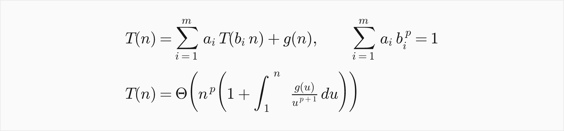
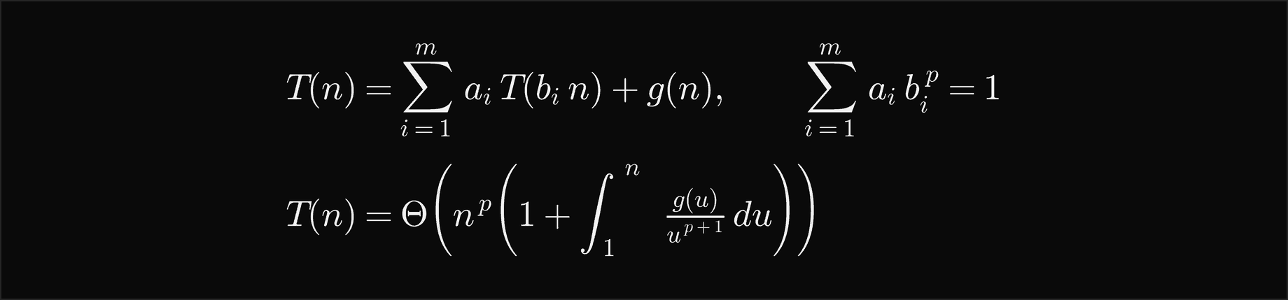
For n/3 and 2n/3, p = 1 and the integral of 1/u is ln n, so T(n) = Θ(n log n), the cost of quicksort with a pivot that always splits one to two. For T(n) = T(n/2) + T(n/4) + n, p = log2 φ = 0.6942 and the root's linear work dominates, Θ(n). For T(n) = 2T(n/2) + T(n/4) + n, p = 1.2716 and the leaves dominate, Θ(n^1.2716). The method also allows each argument to be perturbed by a small amount such as a floor, which is why floors never mattered above. akra_bazzi.py finds p by bisection and evaluates the integral numerically; the pointer is enough here, and the further reading has the proof.

Cost

Summing the levels

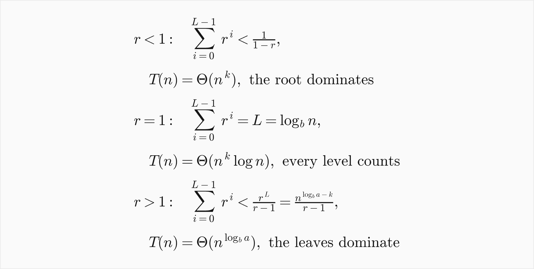
The level sums explain every case of the master theorem. With f(n) = c n^k, level i costs c n^k r^i, where r = a/b^k is the ratio between consecutive levels:

The sum of r^i over the L = log_b n levels is a geometric series, and its size depends only on r:

The example recursion_trees.py computes every level of four recurrences at n = 3^8 = 6561 with T(1) = 1.

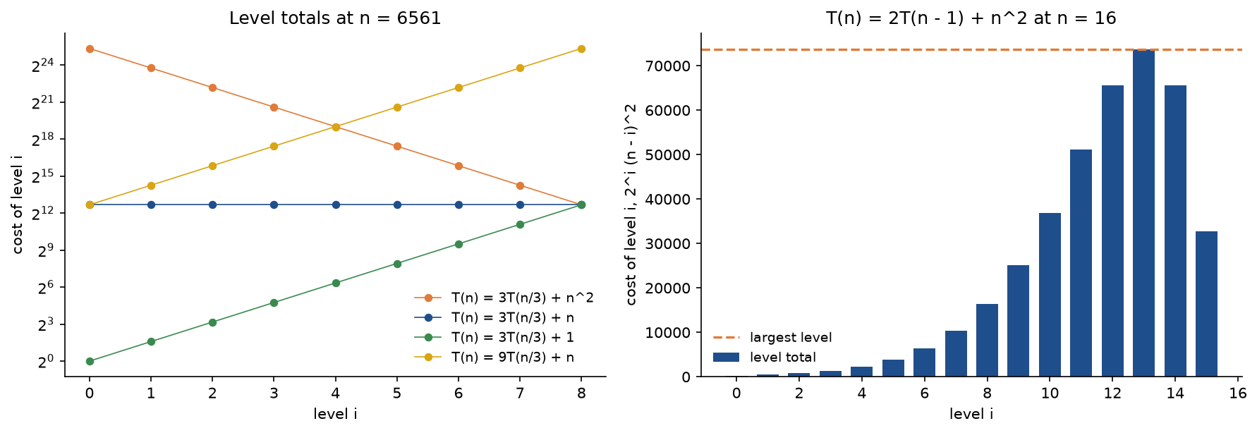
On the left, a straight falling line is case 3, a flat line case 2 and a rising line case 1. The two outer recurrences, 3T(n/3) + n² and 9T(n/3) + n, are mirror images: their level costs are the same numbers in opposite order, so both total (3n² − n)/2 = 64566801, but one spends almost all of it at the root and the other at the leaves. The flat line totals 59049 = n(log3 n + 1), and the leaf-heavy one 9841 = (3n − 1)/2. On the right, the decreasing recurrence's level costs nearly double from level to level until the factor (n − i)² takes over, three levels above the leaves; the last five levels hold almost three quarters of the total 392890. The habit of multiplying the 16 levels by the largest level, 73728, gives 1179648, three times too much, and the factor grows with n.

Counted operations of real code

The recurrences read off the code in the first section are checked against the counters of the running code, for many sizes. Most of them count a worst case: binary search is run with a target smaller than every item, and merge sort's recurrence W(n) bounds its comparisons from above, while its counts on random keys are typical values below that bound. Nothing here is amortized; a recurrence counts every call of one run.

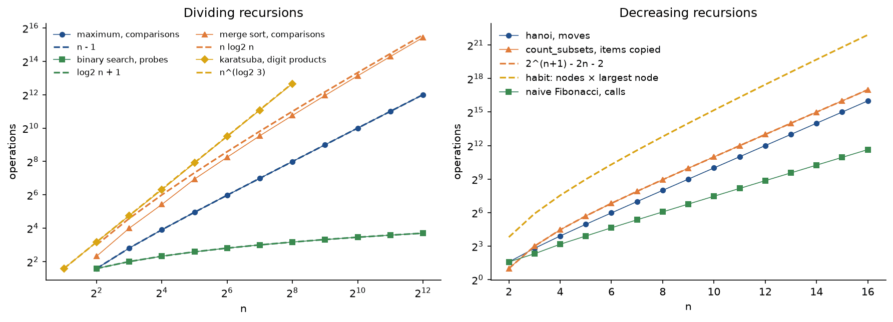
The recursive maximum makes exactly n − 1 comparisons, binary search exactly ⌊log2 n⌋ + 1 probes when the target is smaller than every item, stooge sort exactly the value of its recurrence C(n) = 3C(⌈2n/3⌉) + 1, and merge sort never more than the worst case W(n). Karatsuba's single-digit products stay at or a little below n^(log2 3), 6475 against 6561 at 256 digits, because some halves have leading zeros and so fewer digits. On the right, Hanoi's moves, the subset search's copies and the Fibonacci calls equal 2^n − 1, 2^(n+1) − 2n − 2 and 2F(n + 1) − 1 at every n; at n = 16 the subset search copies 131038 items, while the habit of multiplying its 131071 calls by the largest call's 30 copies would claim 3932130, 30 times as many.

The answers checked against exact values

A Θ answer hides a constant, so it is checked by dividing exact values by the answer and watching the ratio settle. The example master_theorem.py does that for ten recurrences, one or more per case, up to n = 2^60, where on_powers computes T(b^m) level by level.

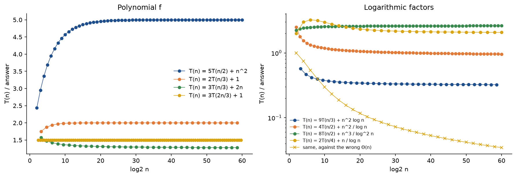
Polynomial answers settle fast: T(n)/n^2.3219 for 5T(n/2) + n² is 4.9539 at n = 2^20 and 5.0000 at 2^60. Logarithmic answers settle slowly, because a logarithm changes slowly: for 4T(n/2) + n²/log n the ratio to n² log log n moves from 1.0638 at 2^20 to 0.9616 at 2^60, still drifting towards its limit ln 2. The amber crosses on the right are the case 3 trap: dividing 2T(n/4) + n/log n by n instead of n/log n gives a ratio that never stops falling.

Stack depth and the cost of evaluating

A recursion uses one stack frame per level of its tree, so the space a recursive function needs is the height of its recursion tree times the space of a frame. Dividing recursions are shallow: merge sort of 16384 items is 15 frames deep, and binary search over 2^40 items 42 deep. Decreasing recursions are as deep as n: Python's recursion limit of about 1000 frames stops a recursive sum over 5000 items with RecursionError. That is why the functions with linear depth in programs.py refuse inputs beyond a stated bound, and why exact.evaluate uses an explicit stack, which evaluates T(n) = T(n − 1) + n³ at n = 20000 without trouble.

Evaluating a recurrence also has a cost. Without a memo table every node of the tree is computed, 2n − 1 evaluations for merge sort's split recurrence at n = 100 and 242785 calls for naive Fibonacci at n = 25. With a memo table only the distinct arguments are computed, and for a dividing recurrence with floors and ceilings those are at most two per level: 33 values for T(10^6).

Worked example

Every step below is printed by examples/worked_example.py and asserted by tests/test_worked_example.py. The main recurrence is T(n) = 3T(n/2) + n with T(1) = 1, the shape of a multiplication that splits each number in half and makes three half-size products, solved at n = 8 by four methods.

Reading the recurrence and unrolling it

Each call on n > 1 does n units of work and makes three calls on n/2; a call on 1 costs 1. Unrolling at n = 8, one line per level:

• T(8) = 8 + 3 T(4)
• = 8 + 12 + 9 T(2)
• = 8 + 12 + 18 + 27 T(1)
• = 8 + 12 + 18 + 27 = 65

Each line multiplies the remaining term by 3 and halves its argument, and each level's cost is 3/2 times the previous one. In general, with n = 2^L, the levels form a geometric series with ratio 3/2 and the base cases add 3^L:

At n = 8 that is 3 · 27 − 16 = 65, and at n = 16 it is 3 · 81 − 32 = 211, matching the unrolling 16 + 24 + 36 + 54 + 81.

The recursion tree

The tree shows the same numbers as levels: one node of cost 8, three of cost 4, nine of cost 2 and twenty-seven leaves of cost 1.

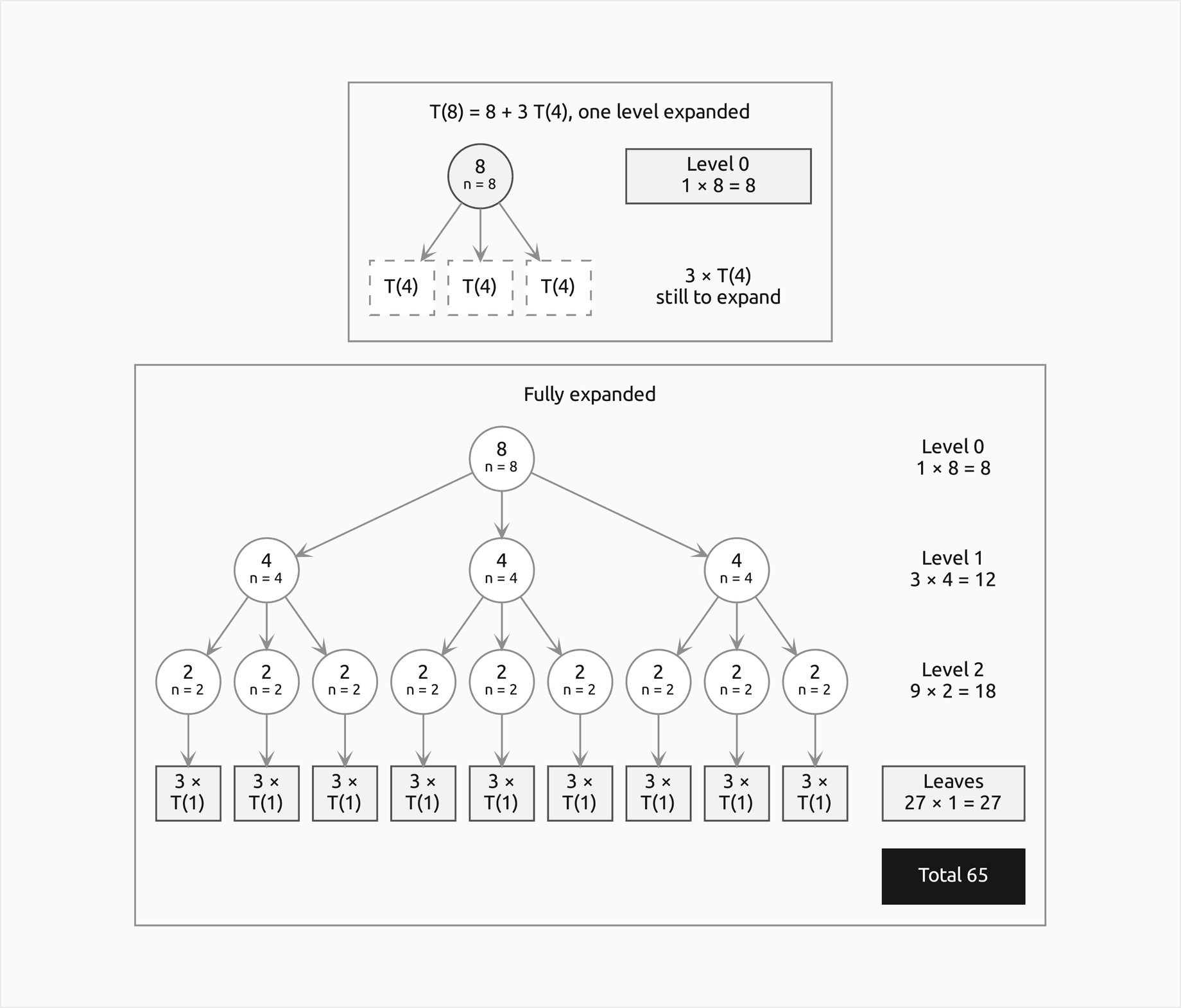
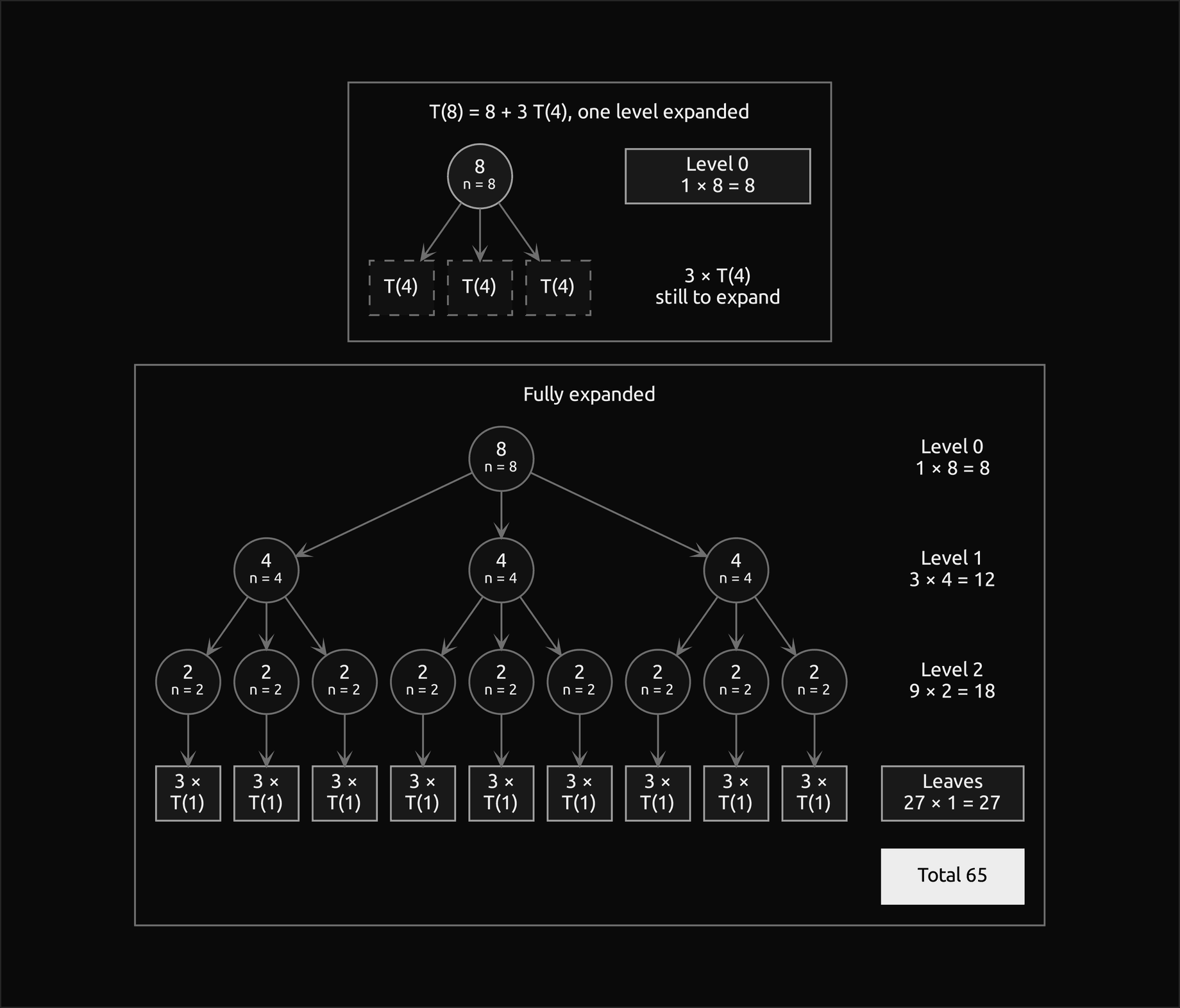
The top frame is the first line of the unrolling, T(8) = 8 + 3T(4); the bottom frame is the last. The level totals 8, 12, 18 and 27 grow by 3/2 per level, so the highlighted leaves are the largest level: this is a leaf-dominated tree, and the answer will be the number of leaves, n^(log2 3).

Proving the bound by substitution

The guess T(n) ≤ c n^(log2 3) is true for c = 3, since T(n) = 3n^(log2 3) − 2n. Its inductive step fails anyway:

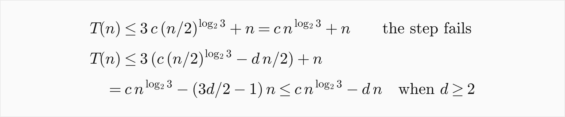
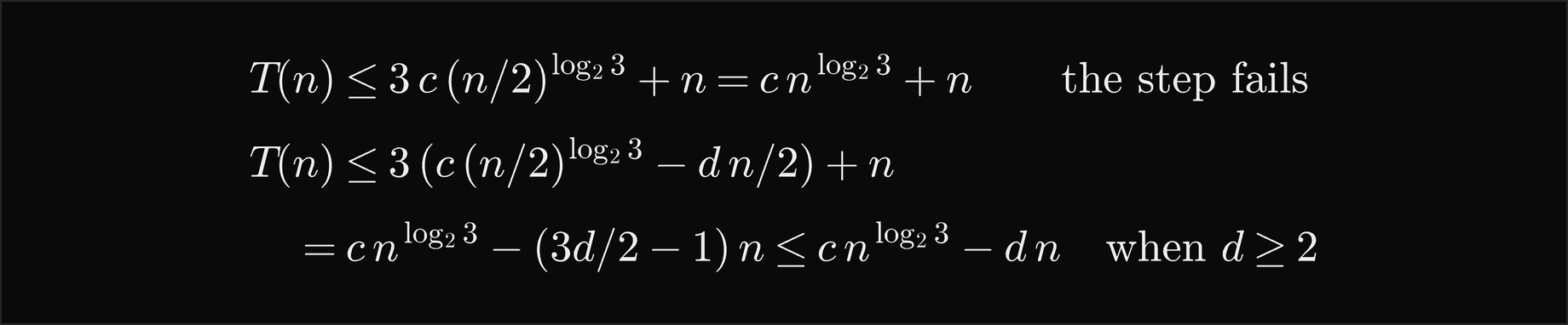
With c = 3 the numbers are:

• assume T(1) ≤ 3; then T(2) ≤ 3 · 3 + 2 = 11, but the claim needs T(2) ≤ 9: fails.
• assume T(2) ≤ 9; then T(4) ≤ 31, but the claim needs ≤ 27: fails.
• assume T(4) ≤ 27; then T(8) ≤ 89, but the claim needs ≤ 81: fails.

Every step overshoots by exactly n. Subtracting the lower-order term 2n fixes it, and the steps then hold with equality:

• base case: T(1) = 1 ≤ 3 · 1 − 2 = 1.
• assume T(1) ≤ 1; then T(2) ≤ 3 · 1 + 2 = 5, and the claim needs ≤ 3 · 3 − 4 = 5: holds.
• assume T(2) ≤ 5; then T(4) ≤ 19, and the claim needs ≤ 27 − 8 = 19: holds.
• assume T(4) ≤ 19; then T(8) ≤ 65, and the claim needs ≤ 81 − 16 = 65: holds.

Equality throughout means the strengthened guess is the exact solution.

The master theorem

The solver prints:

• a = 3, b = 2, critical exponent log_2 3 = 1.5850
• f(n) = n: k = 1, p = 0
• a = 3 > b^k = 2^1 = 2
• case 1: T(n) = Θ(n^1.5850)

The common form agrees: f(n) = n is O(n^(1.5850 − ε)) with ε = 0.5850. The exact values confirm the hidden constant: T(n)/n^(log2 3) is 2.4074 at n = 8, 2.6049 at n = 16 and 2.9994 at n = 2^20, where T(n) = 10458256051, approaching 3 from below because the −2n term fades.

A decreasing recurrence and the habits that overstate it

The second recurrence is T(n) = 2T(n − 1) + n² with T(0) = 0, whose values for n = 0 to 6 are 0, 1, 6, 21, 58, 141 and 318. Unrolling at n = 6 gives the level costs 36, 50, 64, 72, 64 and 32, then 64 base cases of cost 0, which add up to 318. Its tree at n = 4 has the level costs 16, 18, 16 and 8:

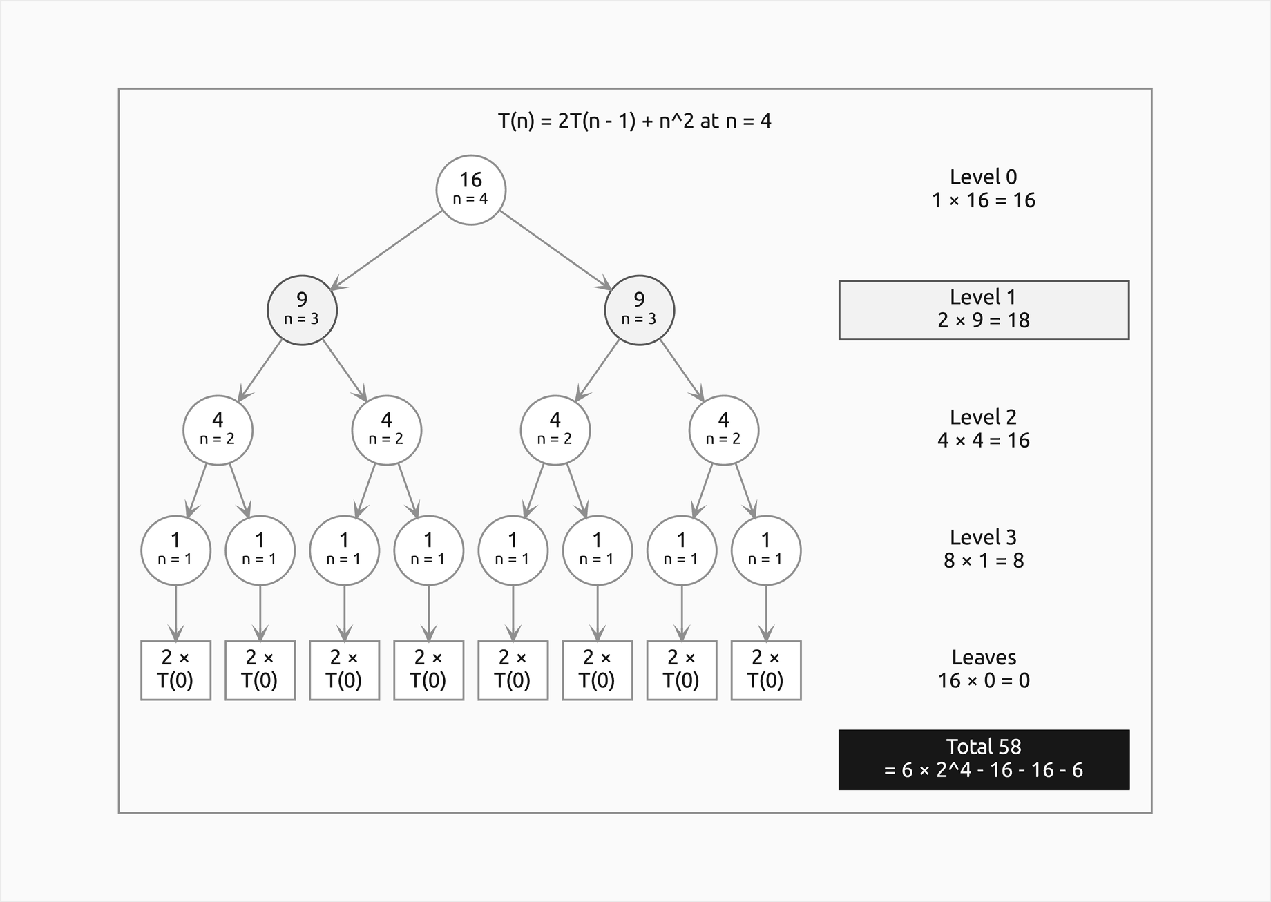
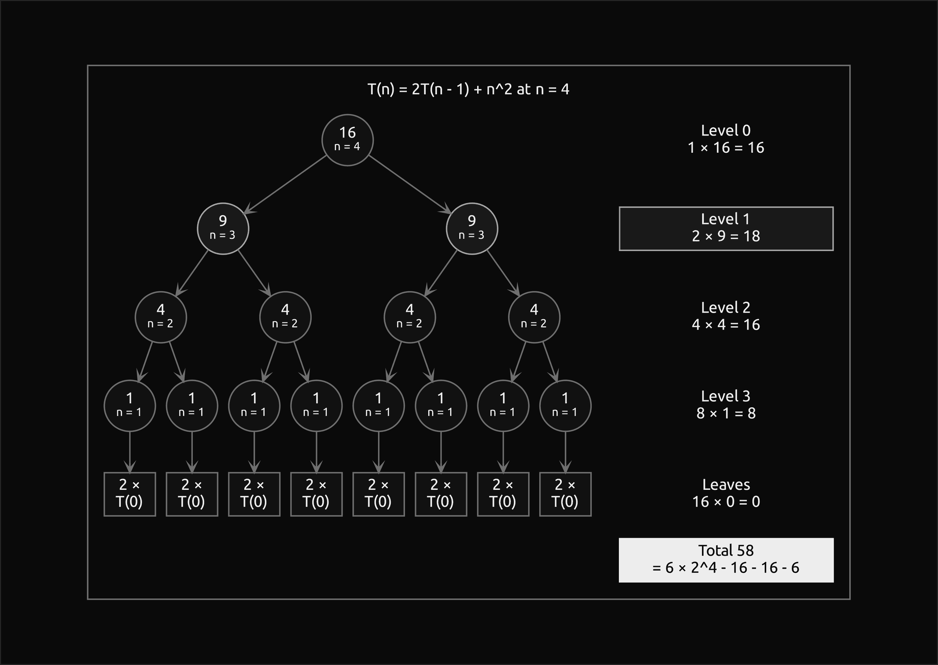
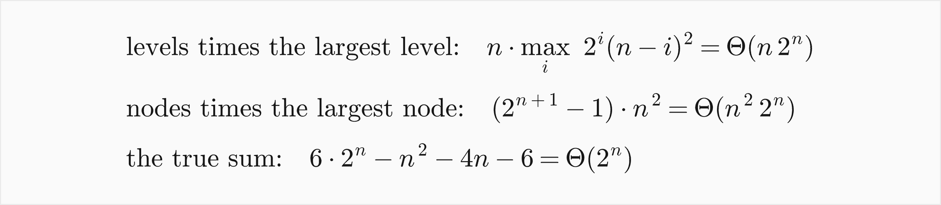
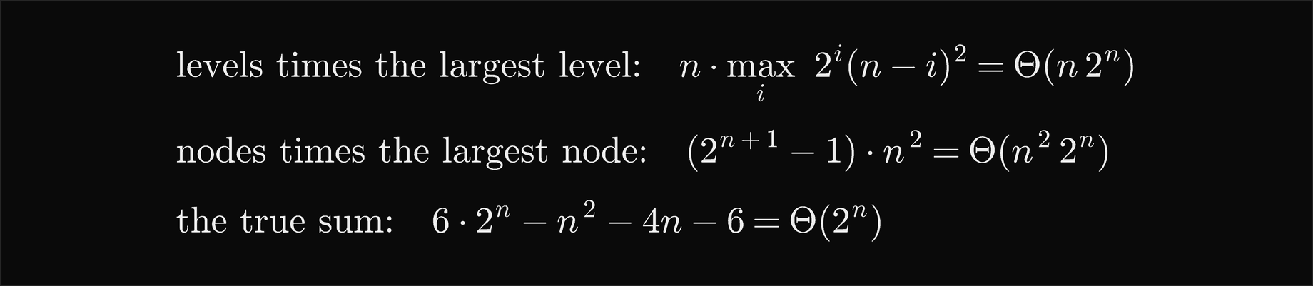
At this small n the heaviest level, highlighted, is level 1; as n grows the heaviest level stays three levels above the leaves, where 2^i keeps doubling while (n − i)² is still 9, and every level above it costs roughly half the one below. Two habits turn that picture into a wrong answer. Multiplying the number of levels by the largest level gives 4 · 18 = 72 here, and Θ(n 2^n) in general; multiplying the number of nodes, 2^(n+1) − 1, by the cost of the largest node, n², gives 31 · 16 = 496 here, and Θ(n² 2^n) in general. The exact sum says otherwise:

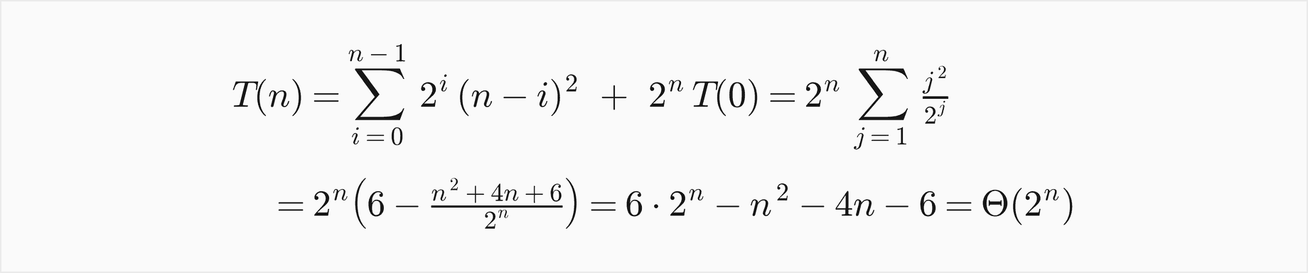
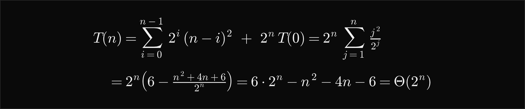
Reindexing by the distance j = n − i from the bottom turns the sum into 2^n times the sum of j²/2^j, which converges to 6, so T(n) = 6 · 2^n − n² − 4n − 6 and neither extra factor appears. Side by side:

• n = 4: exact 58, levels habit 72, nodes habit 496.
• n = 10: exact 5998, levels habit 11520, nodes habit 204700; T(n)/2^n = 5.8574 and T(n)/(n² 2^n) = 0.0586.
• n = 20: exact 6290970, levels habit 23592960, nodes habit 838860400.
• n = 30: exact 6442449918, levels habit 36238786560, nodes habit 1932735282300; T(n)/2^n = 6.0000 and T(n)/(n² 2^n) = 0.0067.

Both habits are upper bounds, but they overstate by factors of about 3n/16 and n²/3 that keep growing: 7.5 and 533 at n = 40. The subset search in programs.py is a program of the same kind, with S(n) = 2S(n − 1) + 2(n − 1): on the first n of the items 5, 3, 8, 2, 7 and 4 it copies 0, 0, 2, 8, 22, 52 and 114 items in 1, 3, 7, 15, 31, 63 and 127 calls, which is 2^(n+1) − 2n − 2, again a constant times 2^n.

A linear recurrence by its characteristic roots

The third recurrence is a_n = a_(n−1) + 12 a_(n−2) with a_0 = 2 and a_1 = 1.

• The characteristic polynomial is x² − x − 12, with the roots 4 and −3, both found exactly among the divisors of 12.
• The general solution is α 4^n + β(−3)^n.
• The initial values give α + β = 2 and 4α − 3β = 1, so α = β = 1.
• So a_n = 4^n + (−3)^n, which grows like Θ(4^n).

The recurrence and the closed form both give 2, 1, 25, 37, 337, 781, 4825 and 14197 for n = 0 to 7.

The code

The package recurrences is plain Python, one idea per module. Importing it needs only the standard library; Matplotlib is imported by plotting.py alone, and NumPy and SciPy only inside the functions of comparisons.py that use them.

• recurrence.py holds recurrences as data: Driving for f(n) = c n^k log^p n, Dividing for aT(n/b) + f(n) with exact, floor, ceiling or split arguments, Decreasing for aT(n − b) + f(n), and General for anything else, all with the same terms, cost, is_base and text methods.
• exact.py holds evaluate, the ground truth, with a memo table and an explicit stack; evaluate_without_memo; on_powers, which reaches n = 2^60 level by level; and ratios and settles for checking a Θ answer.
• unrolling.py holds unroll, which prints the lines of back substitution, geometric_closed_form, decreasing_sum and the checked CLOSED_FORMS.
• trees.py holds recursion_tree, level_costs, levels_of and shape, which says whether the root, every level or the leaves dominate.
• substitution.py holds Bound, inductive_step, check_induction, first_failure and bound_holds, which separate a bound that is true from one whose induction goes through.
• master.py holds common_master, extended_master, the regularity checks and report; decreasing.py holds decreasing_master and the loose bound; akra_bazzi.py holds the exponent, the integral and uneven recurrences; failures.py holds the recurrences the theorem does not cover; floors.py holds the rounded recurrences and the sandwich check.
• roots.py finds characteristic roots, integer ones exactly and the rest by the quadratic formula or the Durand-Kerner iteration; linear.py holds solve_linear, which fixes the weights by Gaussian elimination; fibonacci.py holds Fibonacci numbers, Binet's formula, the naive recursion and Euclid's algorithm with Lamé's bounds.
• programs.py holds the instrumented recursive functions on sequences: the recursive maximum, binary search, merge sort, stooge sort, Towers of Hanoi and the subset search; multiplication.py holds Karatsuba's multiplication, the plain four-product split and power by squaring.
• instrument.py holds CallRecorder, which turns any instrumented run into a call tree with each call's own and total work.
• counting.py holds OperationCounter with the fields calls, steps, comparisons, multiplications, additions and evaluations, and CountedKey; trace.py holds the Step record and format_trace.
• invariants.py holds hypotheses_violation, closed_form_violation, level_sum_violation and call_tree_violation, each with its is_ and check_ forms.
• workloads.py holds the worked example, the seeded random recurrences, linear recurrences and inputs, whose generators draw from fixed parameter ranges so that every generated recurrence and exercise is a fresh instance; layout.py places the nodes of a recursion tree with a tidy layout that centres each parent over its children, frames.py measures each pictured state with its level column, and drawing.py pins them in deterministic Graphviz text; comparisons.py puts the library tools next to the package; pitfalls.py holds the wrong habits; plotting.py draws every figure in the handbook's colours.

A recorded call is two lines around the body of a function, and the counter does the rest:

enter(recorder, "maximum", hi - lo)
counter.calls += 1
if hi - lo == 1:
    result = values[lo]
else:
    middle = (lo + hi + 1) // 2
    left = maximum_between(values, lo, middle, counter, recorder)
    right = maximum_between(values, middle, hi, counter, recorder)
    counter.comparisons += 1
    result = right if left < right else left
leave(recorder)

The examples run in a few seconds each from the repository root:

• examples/worked_example.py prints every step of the worked example and writes its two diagram sources.
• examples/recursion_trees.py draws the three trees, plots the level costs and checks the recurrences of real code against counted runs.
• examples/master_theorem.py runs the solver on every case, the decreasing form, Akra-Bazzi, the failures and the floors.
• examples/linear_recurrences.py solves linear recurrences with distinct, repeated and complex roots, and covers Fibonacci and Euclid.
• examples/common_mistakes.py runs every wrong habit from pitfalls.py next to the right answer.
• examples/compare_with_libraries.py checks the package against functools.cache, math.log, NumPy and SciPy.
• examples/practice.py prints fresh exercises with their solutions; --seed gives a new set.

python foundations/recurrences/examples/worked_example.py
python foundations/recurrences/examples/recursion_trees.py
python foundations/recurrences/examples/master_theorem.py
python foundations/recurrences/examples/linear_recurrences.py
python foundations/recurrences/examples/common_mistakes.py
python foundations/recurrences/examples/compare_with_libraries.py
python foundations/recurrences/examples/practice.py --seed 7

The sample project, project/analyse_recursion.py with its helper project/inference.py, is a recurrence analyser for recursive Python functions. For each of nine functions, from merge sort, Karatsuba and binary search to naive Fibonacci and the subset search, it records the call tree of one large run and infers the recurrence from the tree alone: a is the typical number of calls a call makes, the sizes shrink either by a factor b (the median ratio of a parent's size to a child's, read from the larger calls and snapped to a simple fraction such as 3/2) or by a fixed difference, and f(n) = c n^k is a least-squares line through the logarithms of each call's own work against its size. It then predicts the growth of the work and of the number of calls with the extended master theorem, the decreasing form or the characteristic roots, measures both over a range of sizes, and reports the ratio of measured to predicted, its drift over the larger sizes and the slope of the measured against the predicted values on log-log axes. Options --functions, --seed, --show-tree and --figures change the run, and the default run takes a few seconds.

python foundations/recurrences/project/analyse_recursion.py
python foundations/recurrences/project/analyse_recursion.py --functions karatsuba,stooge_sort --show-tree 3

The analyser recovers every recurrence. For merge sort it infers 2T(n/2) + 0.94n and Θ(n log n); for Karatsuba 3T(n/2) + 9.29n and Θ(n^1.5850); for stooge sort 3T(2n/3) + 1 and Θ(n^2.7095); for naive Fibonacci calls on n − 1 and n − 2 and Θ(1.6180^n); and for the subset search 2T(n − 1) + 1.76n, close to its true own work 2(n − 1), and Θ(2^n), with measured over predicted settling at 1.9995, while against the habit n 2^n the same counts drift from 0.3438 down to 0.1250.

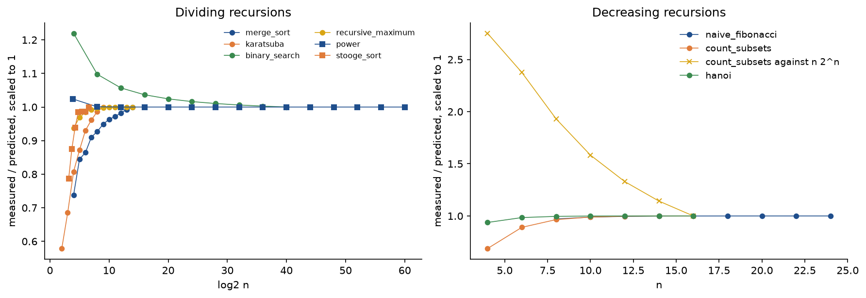
A flat line at 1 means the prediction has the right growth; the constant it hides is the level the unscaled ratio settles at. The ratios approach 1 from below or above as lower-order terms fade: binary search's ⌊log2 n⌋ + 1 probes against log2 n, merge sort's n log2 n − 1.25n or so comparisons against n log2 n. Stooge sort is measured at 9, 13, 19, 28, 42, 63 and 94, sizes that follow its ceilings exactly; between them its count is a staircase, which the floors section explains.

The notebook recurrences.ipynb follows this page: the worked example step by step, the trees and level costs, the solver on every case, the failures, floors and ceilings, linear recurrences, the comparison with the libraries and a short run of the analyser. The tests in tests check the worked example value by value, every closed form, the level sums, the solver against exact values on hundreds of seeded random recurrences, every instrumented function against its recurrence, the call trees, and the agreement with functools.cache, NumPy and SciPy, and run in a few seconds:

python -m pytest foundations/recurrences

All data are synthetic, generated from seeds by workloads.py and the project, so nothing is downloaded and no licence is involved.

In practice

Exact values with functools.cache and Fraction

The quickest way to check a recurrence in Python is to write it as a function and let functools.cache remember the values:

from functools import cache


@cache
def merge_steps(n: int) -> int:
    return 0 if n <= 1 else merge_steps((n + 1) // 2) + merge_steps(n // 2) + n

comparisons.cached_evaluate does this for any recurrence of the package and agrees with exact.evaluate value for value, including the number of distinct values computed: 33 for the split recurrence at n = 10^6, 31 for 5T(n/2) + n² at n = 2^30. The cached version recurses in Python, so it suits recurrences with logarithmic depth; for decreasing ones the explicit stack of exact.evaluate or a plain loop is safer. Python's integers are exact at any size, which is why the package can compare T(2^20) = 10458256051 with a closed form digit for digit, and fractions.Fraction keeps rational arguments such as 2n/3 exact.

Roots, exponents and matrix powers from NumPy and SciPy

numpy.roots finds characteristic roots as the eigenvalues of the companion matrix, and agrees with the package to about 1e-16 on distinct roots. On the double root of x² − 12x + 36 it is off by 7.5e-08, the usual loss of accuracy at repeated roots, while the package finds 6 exactly by trying the divisors of 36. NumPy's matrix_power on an object array of Python integers computes F(n) exactly from the n-th power of [[1, 1], [1, 0]], in O(log n) matrix products. scipy.optimize.brentq finds the Akra-Bazzi exponent and agrees with the package's bisection to within 1e-15; math.log(a, b) gives the critical exponent. Counted through CountedKey, Python's sorted makes 8623 comparisons on 1000 random keys against 8753 for the package's merge sort, both a little below n log2 n = 9966, and in wall-clock time it is roughly 15 to 20 times faster, the usual gap between C and Python. When to use which:

• Use functools.cache or a loop to tabulate a recurrence and test a guess on concrete numbers before trying to prove it.
• Use the master theorem, in the extended form when f has logarithms, for any balanced divide-and-conquer recurrence; use the decreasing form for recursions that peel off a constant.
• Use characteristic roots for linear recurrences with constant coefficients, and NumPy when the roots are not integers.
• Use Akra-Bazzi for uneven splits, and a recursion tree or substitution when nothing else applies.

Computer algebra and other tools

SymPy's rsolve and Mathematica's RSolve solve linear recurrences symbolically, including non-homogeneous ones; Mathematica also handles many divide-and-conquer recurrences on powers of b. Analysers that guess growth from measurements, such as the sample project, are the empirical side of the same idea, and profilers report call counts that can be compared with a recurrence. Languages with tail-call elimination, such as Scheme and many functional languages, run a tail-recursive decreasing recursion in constant stack space; Python, Java and most C compilers in debug builds do not, so deep decreasing recursions are rewritten as loops there.

Pitfalls

• Multiplying the number of levels by the largest level, or the number of nodes by the largest node. Both are valid upper bounds but not the answer when level costs grow geometrically: for T(n) = 2T(n − 1) + n² they claim Θ(n 2^n) and Θ(n² 2^n) while the truth is 6 · 2^n − n² − 4n − 6, too much by factors of 7.5 and 533 at n = 40. Sum the levels; examples/common_mistakes.py runs this and every following mistake.
• Writing O(n^k a^(n/b)) for a decreasing recurrence with a > 1. The polynomial factor disappears into the converging series, and the answer is Θ(a^(n/b)).
• Dropping the logarithm in case 3 when p < 0. T(n) = 2T(n/4) + n/log n is Θ(n/log n), not Θ(n); the ratio T(n)/n falls from 0.1168 to 0.0346 between n = 4^10 and 4^30.
• Treating log n as a polynomial factor. 3T(n/3) + n log n is not case 3 of the common form, and the answer Θ(n log n) is short by a log factor: the ratio to n log2 n grows from 3.6052 to 18.5175 between n = 3^6 and 3^36. The extended form gives Θ(n log² n).
• Swapping log_b a and log_a b. For 5T(n/2) + n², log_5 2 = 0.4307 suggests case 3 and Θ(n²), while log_2 5 = 2.3219 gives case 1 and Θ(n^2.3219); write b as the base every time.
• Applying the theorem outside its hypotheses: a that depends on n, a below 1, a negative or decreasing f, or a case 3 driving function that fails regularity. Check the hypotheses first, as hypotheses_violation does.
• Proving T(n) ≤ cn when the inductive step gives cn + 1. The bound may be true, but this induction cannot show it; subtract a lower-order term from the guess, as the recursive maximum and the worked example show.
• Letting the constant grow in an induction. Deriving T(n) ≤ cn + n and calling it O(n) proves nothing; the constant in the conclusion must be the constant in the hypothesis.
• Charging every level the top level's cost while unrolling. Writing C(n − k) + k(n − 1) for selection sort's C(n) = C(n − 1) + n − 1 gives a correct final O(n²) through false intermediate lines (81 instead of 45 for the last nine levels at n = 10); keep each level's own cost.
• Forgetting the work hidden in one expression. A slice, a concatenation or a membership test on a list costs time proportional to its length, as the subset search's two items[1:] slices do; read every line of the code as an operation count.
• Recursing to depth n in Python. A recursive sum over 5000 items raises RecursionError at the default limit of about 1000 frames; use a loop or an explicit stack, as exact.evaluate does.
• Trusting a closed form that was never checked. Compute the recurrence for small n and compare; a mistake in the base case or one off-by-one in the exponent shows at once.

Further reading

• T. H. Cormen, C. E. Leiserson, R. L. Rivest and C. Stein, Introduction to Algorithms, fourth edition, chapter 4, MIT Press, 2022. The substitution method, recursion trees, the master theorem with its regularity condition, and Akra-Bazzi.
• J. L. Bentley, D. Haken and J. B. Saxe, "A general method for solving divide-and-conquer recurrences", ACM SIGACT News 12(3), 36-44, 1980. The origin of the master theorem.
• M. Akra and L. Bazzi, "On the solution of linear recurrence equations", Computational Optimization and Applications 10(2), 195-210, 1998.
• T. Leighton, "Notes on better master theorems for divide-and-conquer recurrences", MIT, 1996. A short proof of Akra-Bazzi and the perturbation result that covers floors and ceilings.
• R. L. Graham, D. E. Knuth and O. Patashnik, Concrete Mathematics, second edition, chapters 1, 6 and 7, Addison-Wesley, 1994. Recurrences, Fibonacci numbers and generating functions.
• D. E. Knuth, The Art of Computer Programming, volume 2, Seminumerical Algorithms, third edition, sections 4.3.3 and 4.5.3, Addison-Wesley, 1997. Fast multiplication and the analysis of Euclid's algorithm.
• G. Lamé, "Note sur la limite du nombre des divisions dans la recherche du plus grand commun diviseur entre deux nombres entiers", Comptes rendus de l'Académie des sciences 19, 867-870, 1844.
• A. Karatsuba and Yu. Ofman, "Multiplication of many-digital numbers by automatic computers", Proceedings of the USSR Academy of Sciences 145, 293-294, 1962.
• R. Sedgewick and P. Flajolet, An Introduction to the Analysis of Algorithms, second edition, chapter 2, Addison-Wesley, 2013. Recurrences of every kind that the analysis of algorithms produces.